Computational Finance Zvi Wiener 02 588 3049 http

Computational Finance Zvi Wiener 02 588 3049 http: //pluto. mscc. huji. ac. il/~mswiener/zvi. html CF 1 Bank Hapoalim Jun 2001

Plan. 1 Introduction, deterministic methods. . 2 Stochastic methods. . 3 Monte Carlo I. . 4 Monte Carlo II. . 5 Advanced methods for derivatives. Other topics: queuing theory, floaters, binomial trees, numeraire, ESPP, convertible bond, DAC, ML CHKP. Zvi Wiener CF 1 2

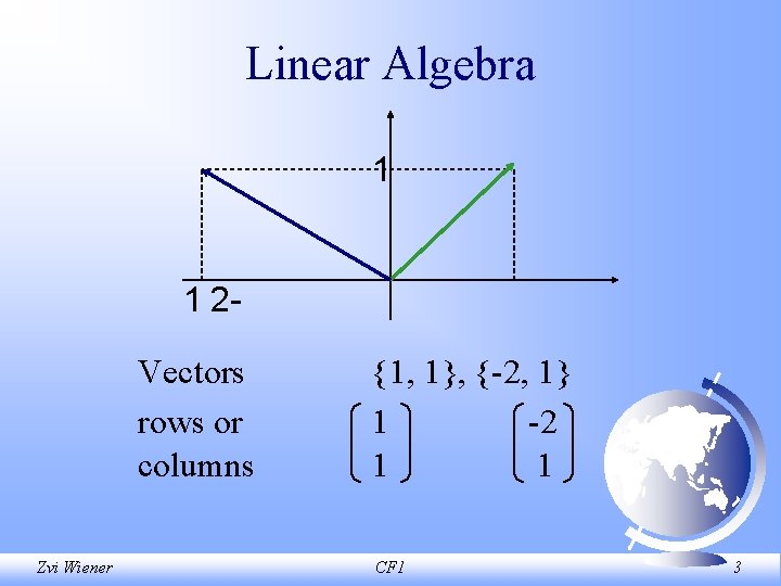
Linear Algebra 1 1 2 Vectors rows or columns Zvi Wiener {1, 1}, { 2, 1} 1 2 1 1 CF 1 3

Linear Algebra Zvi Wiener CF 1 4

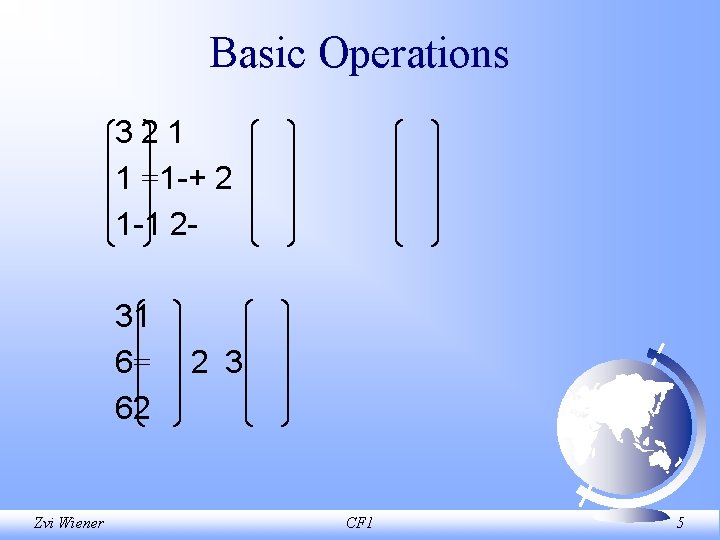
Basic Operations 321 1 =1 -+ 2 1 -1 231 6= 62 Zvi Wiener 2 3 CF 1 5

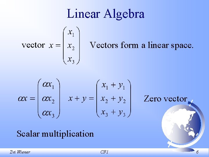
Linear Algebra vector Vectors form a linear space. Zero vector Scalar multiplication Zvi Wiener CF 1 6

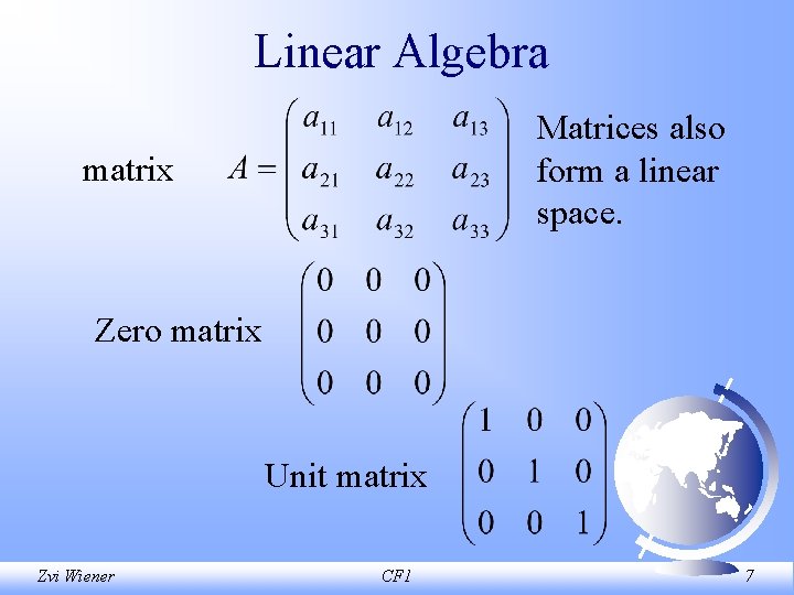
Linear Algebra Matrices also form a linear space. matrix Zero matrix Unit matrix Zvi Wiener CF 1 7

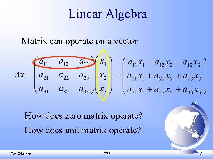
Linear Algebra Matrix can operate on a vector How does zero matrix operate? How does unit matrix operate? Zvi Wiener CF 1 8

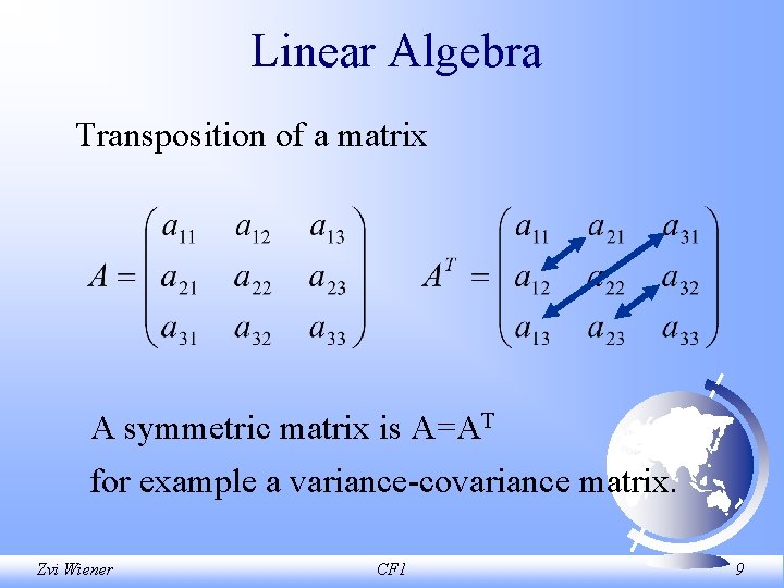
Linear Algebra Transposition of a matrix A symmetric matrix is A=AT for example a variance covariance matrix. Zvi Wiener CF 1 9

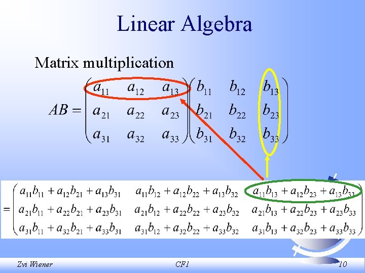
Linear Algebra Matrix multiplication Zvi Wiener CF 1 10

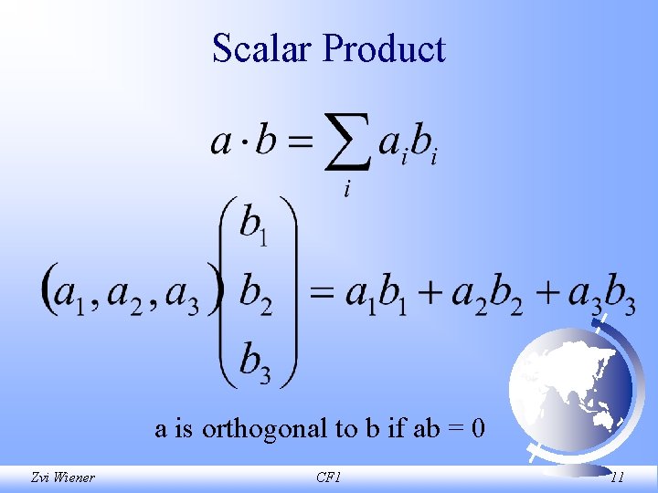
Scalar Product a is orthogonal to b if ab = 0 Zvi Wiener CF 1 11

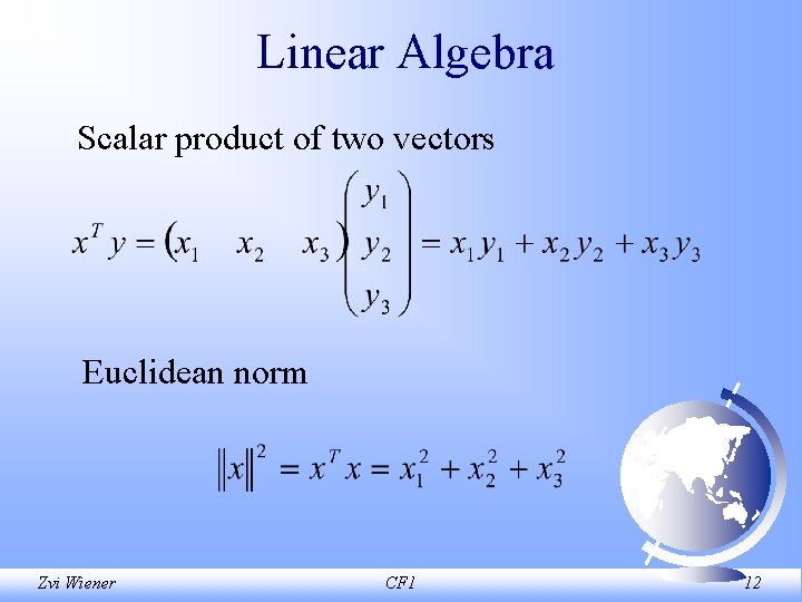
Linear Algebra Scalar product of two vectors Euclidean norm Zvi Wiener CF 1 12

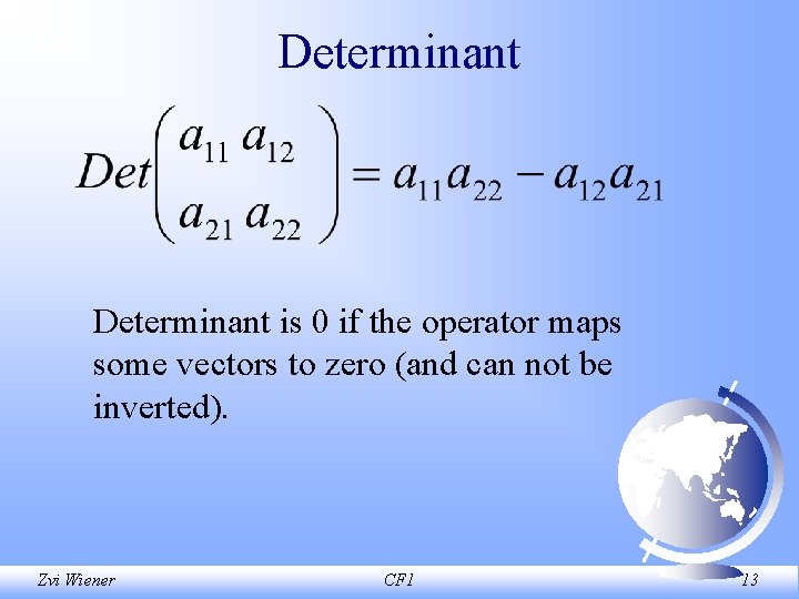
Determinant is 0 if the operator maps some vectors to zero (and can not be inverted). Zvi Wiener CF 1 13

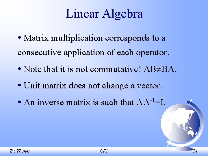
Linear Algebra • Matrix multiplication corresponds to a consecutive application of each operator. • Note that it is not commutative! AB BA. • Unit matrix does not change a vector. • An inverse matrix is such that AA 1=I. Zvi Wiener CF 1 14

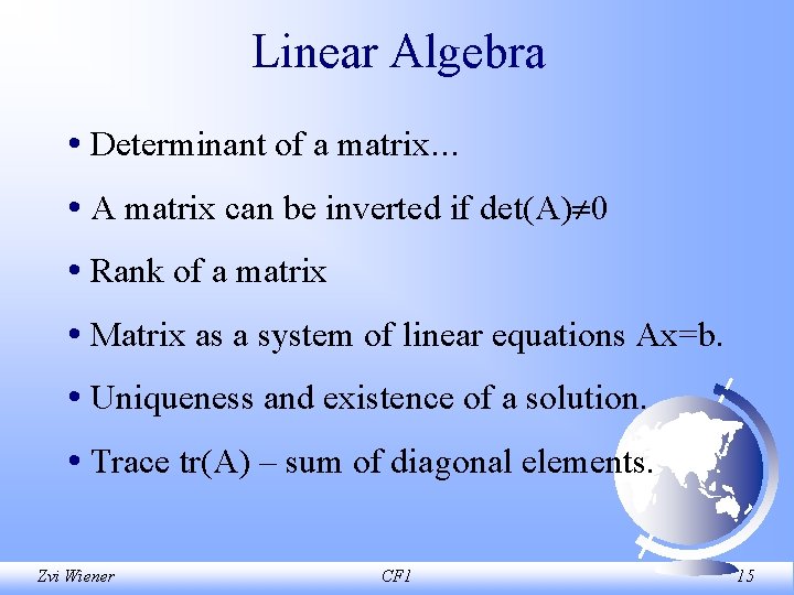
Linear Algebra • Determinant of a matrix. . . • A matrix can be inverted if det(A) 0 • Rank of a matrix • Matrix as a system of linear equations Ax=b. • Uniqueness and existence of a solution. • Trace tr(A) – sum of diagonal elements. Zvi Wiener CF 1 15

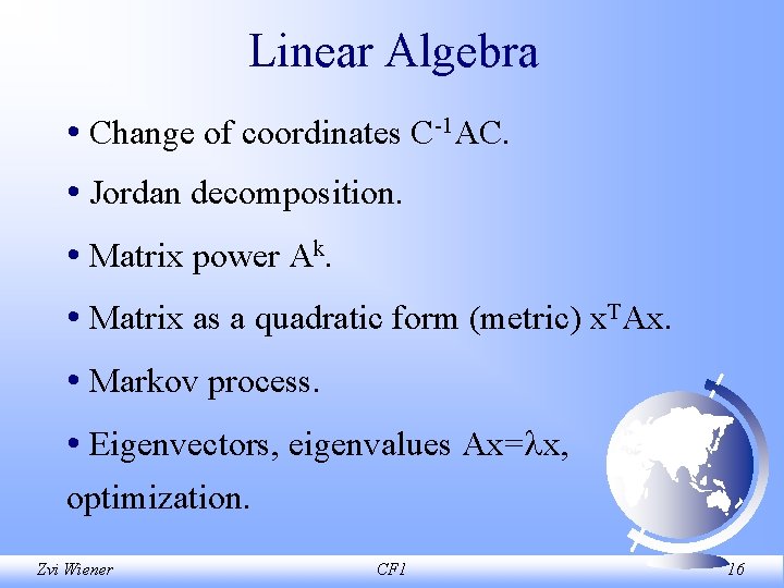
Linear Algebra • Change of coordinates C 1 AC. • Jordan decomposition. • Matrix power Ak. • Matrix as a quadratic form (metric) x. TAx. • Markov process. • Eigenvectors, eigenvalues Ax= x, optimization. Zvi Wiener CF 1 16

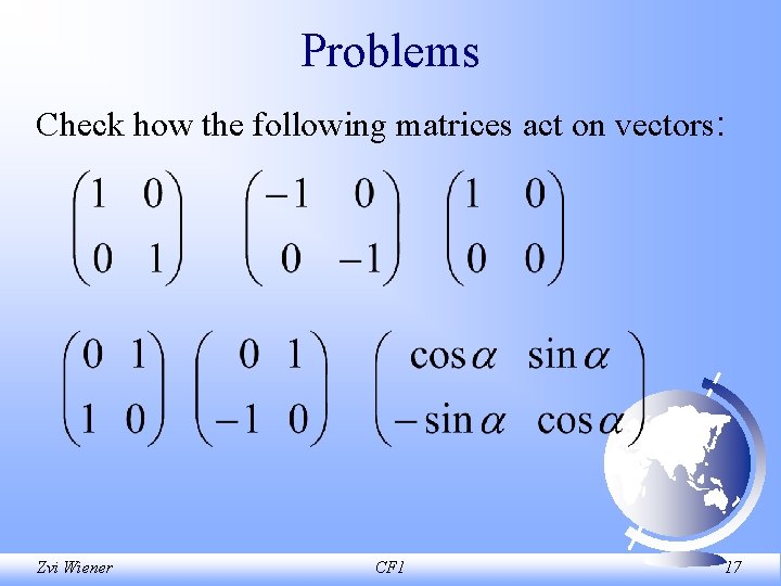
Problems Check how the following matrices act on vectors: Zvi Wiener CF 1 17

Simple Exercises • Show an example of AB BA. • Construct a matrix that inverts each vector. • Construct a matrix that rotates a two dimensional vector by an angle . • Construct a covariance matrix, show that it is symmetric. • What is mean and variance of a portfolio in matrix terms? Zvi Wiener CF 1 18

Examples • Credit rating and credit dynamics. • Variance covariance model of Va. R. • Can the var-covar matrix be inverted • Va. R isolines (the ovals model. ( • Prepayment model based on types of clients. • Finding a minimum of a function. Zvi Wiener CF 1 19

Calculus • Function of one and many variables. • Continuity in one and many directions. • Derivative and partial derivative. • Gradient and Hessian. • Singularities, optimization, ODE, PDE. Zvi Wiener CF 1 20

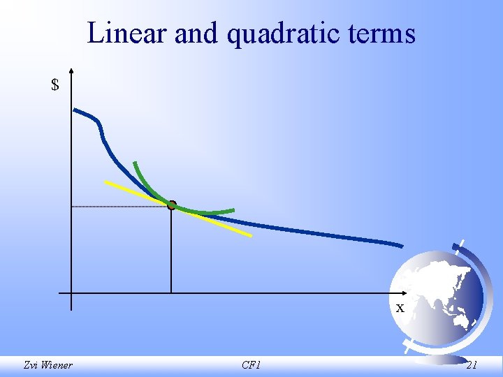
Linear and quadratic terms $ x Zvi Wiener CF 1 21

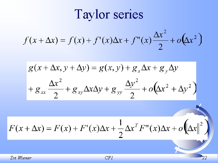
Taylor series Zvi Wiener CF 1 22

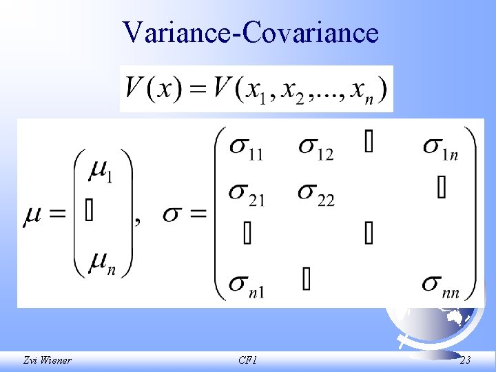
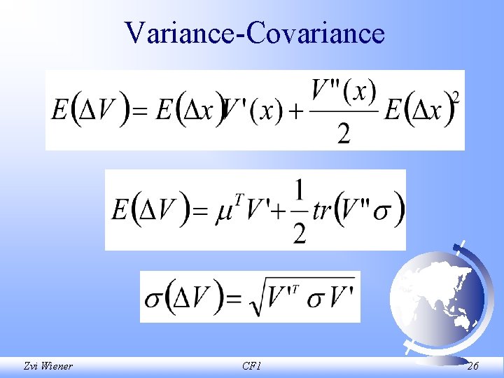
Variance Covariance Zvi Wiener CF 1 23

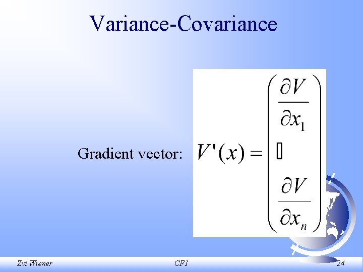
Variance Covariance Gradient vector: Zvi Wiener CF 1 24

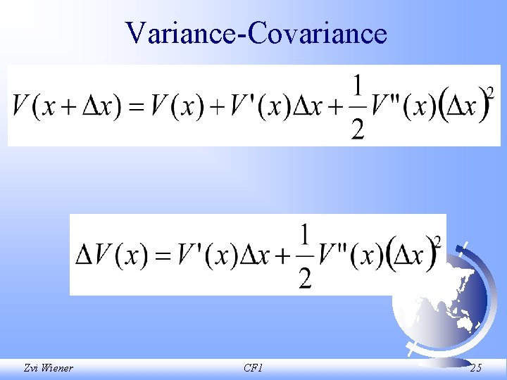
Variance Covariance Zvi Wiener CF 1 25

Variance Covariance Zvi Wiener CF 1 26

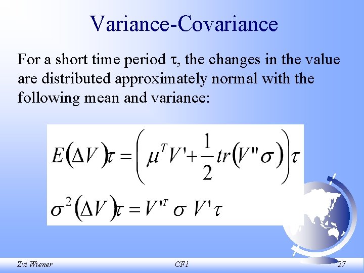
Variance Covariance For a short time period , the changes in the value are distributed approximately normal with the following mean and variance: Zvi Wiener CF 1 27

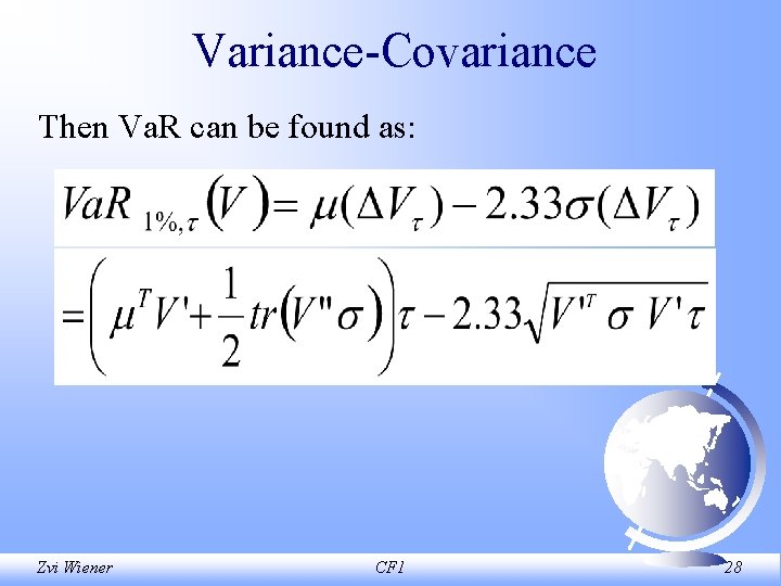
Variance Covariance Then Va. R can be found as: Zvi Wiener CF 1 28

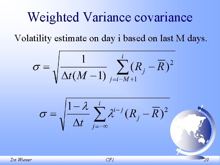
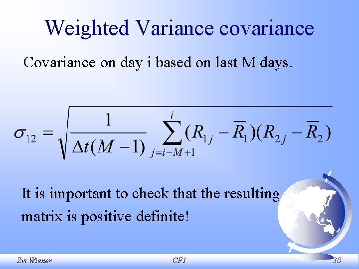
Weighted Variance covariance Volatility estimate on day i based on last M days. Zvi Wiener CF 1 29

Weighted Variance covariance Covariance on day i based on last M days. It is important to check that the resulting matrix is positive definite! Zvi Wiener CF 1 30

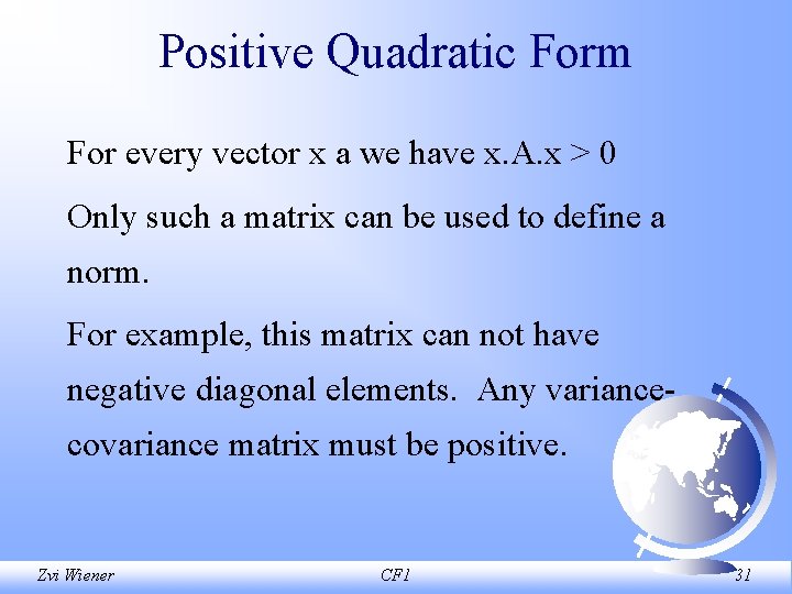
Positive Quadratic Form For every vector x a we have x. A. x > 0 Only such a matrix can be used to define a norm. For example, this matrix can not have negative diagonal elements. Any variance covariance matrix must be positive. Zvi Wiener CF 1 31

Positive Quadratic Form Needs["Linear. Algebra`Matrix. Manipulation`"]; Clear. All[ positive. Form ]; positive. Form[ a_? Matrix. Q ] : = Module[{aa, i}, aa = Table[ Det[ Take. Matrix[ a, {1, 1}, {i, i}] ], {i, Length[a]}]; { aa, If[ Count[ aa, t_ /; t < 0] > 0, False, True]} ]; Zvi Wiener CF 1 32

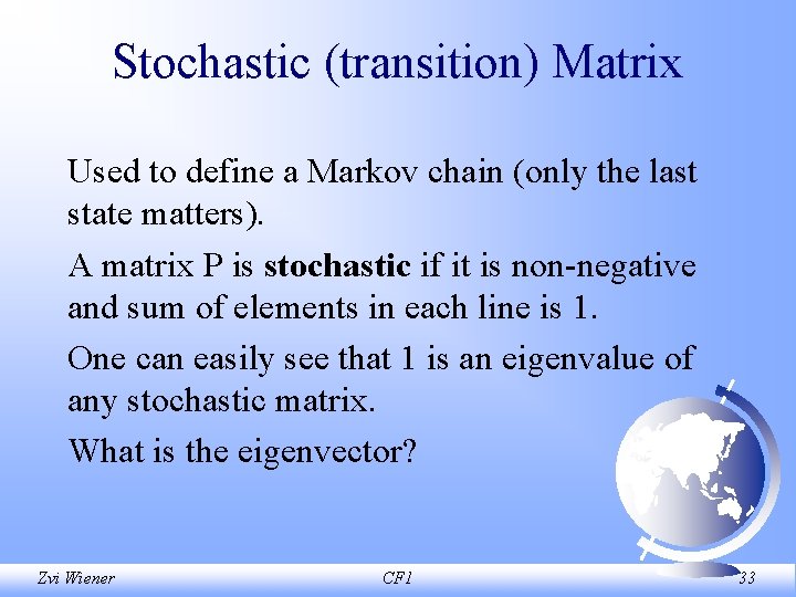
Stochastic (transition) Matrix Used to define a Markov chain (only the last state matters). A matrix P is stochastic if it is non negative and sum of elements in each line is 1. One can easily see that 1 is an eigenvalue of any stochastic matrix. What is the eigenvector? Zvi Wiener CF 1 33

Markov chain • credit migration • prepayment and freezing of a program Zvi Wiener CF 1 34

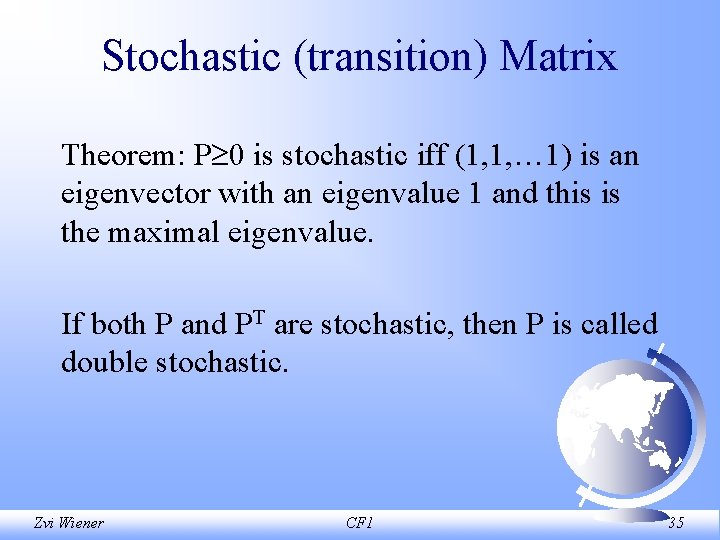
Stochastic (transition) Matrix Theorem: P 0 is stochastic iff (1, 1, … 1) is an eigenvector with an eigenvalue 1 and this is the maximal eigenvalue. If both P and PT are stochastic, then P is called double stochastic. Zvi Wiener CF 1 35

Cholesky decomposition The Cholesky decomposition writes a symmetric positive definite matrix as the product of an upper triangular matrix and its transpose. In MMA Zvi Wiener Cholesky. Decomposition[m] CF 1 36

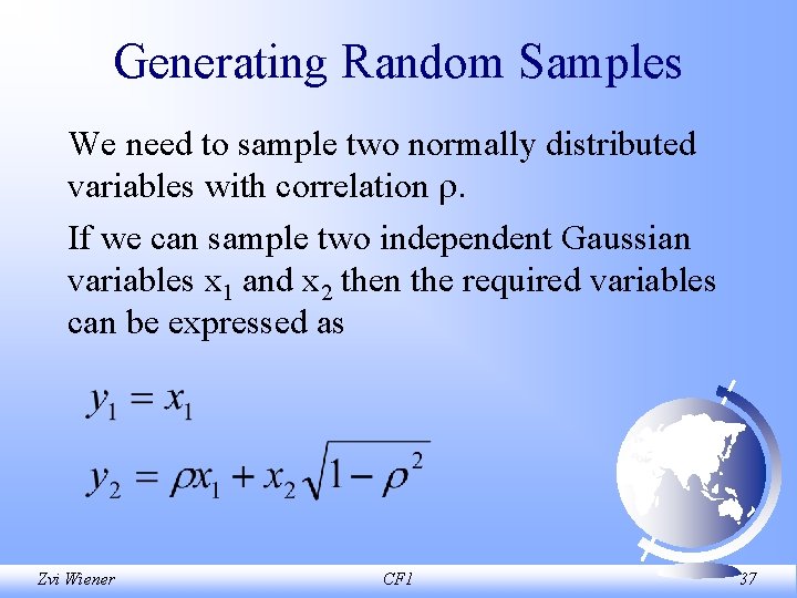
Generating Random Samples We need to sample two normally distributed variables with correlation . If we can sample two independent Gaussian variables x 1 and x 2 then the required variables can be expressed as Zvi Wiener CF 1 37

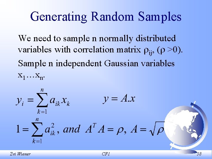
Generating Random Samples We need to sample n normally distributed variables with correlation matrix ij, ( >0). Sample n independent Gaussian variables x 1…xn. Zvi Wiener CF 1 38

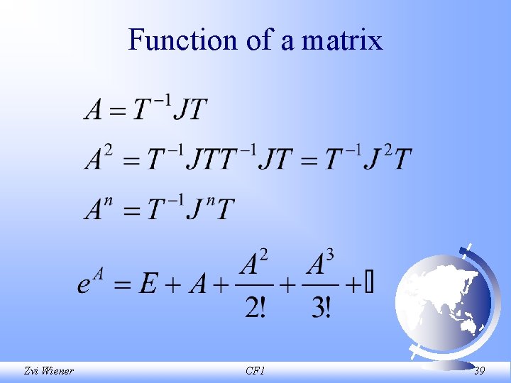
Function of a matrix Zvi Wiener CF 1 39

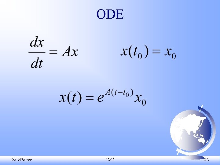
ODE Zvi Wiener CF 1 40

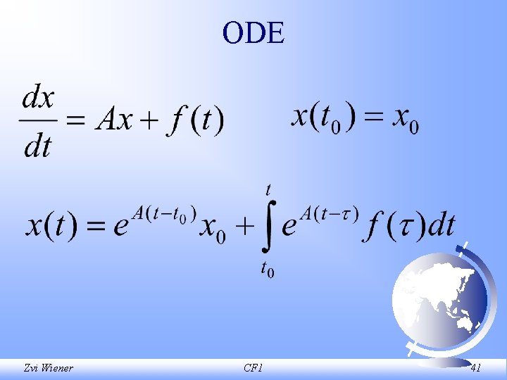
ODE Zvi Wiener CF 1 41

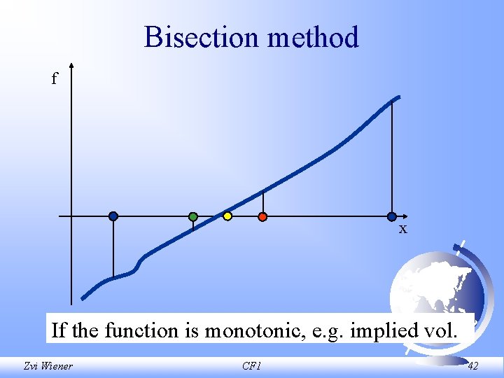
Bisection method f x If the function is monotonic, e. g. implied vol. Zvi Wiener CF 1 42

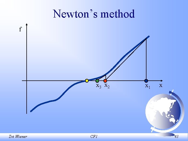
Newton’s method f x 3 x 2 Zvi Wiener CF 1 x 43

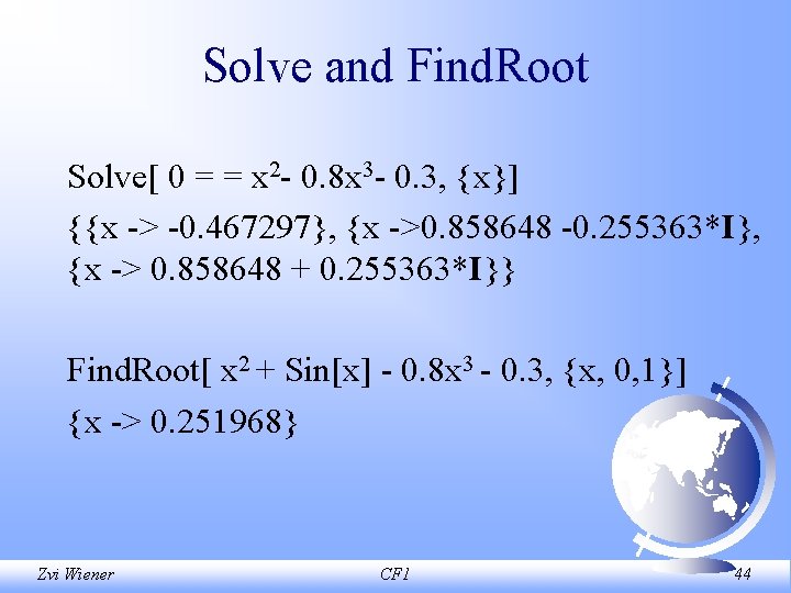
Solve and Find. Root Solve[ 0 = = x 2 0. 8 x 3 0. 3, {x}] {{x > 0. 467297}, {x >0. 858648 0. 255363*I}, {x > 0. 858648 + 0. 255363*I}} Find. Root[ x 2 + Sin[x] 0. 8 x 3 0. 3, {x, 0, 1}] {x > 0. 251968} Zvi Wiener CF 1 44

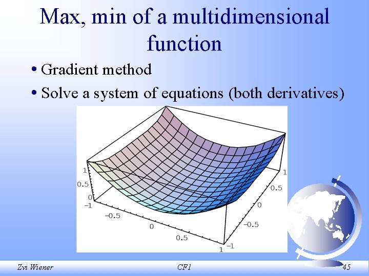
Max, min of a multidimensional function • Gradient method • Solve a system of equations (both derivatives) Zvi Wiener CF 1 45

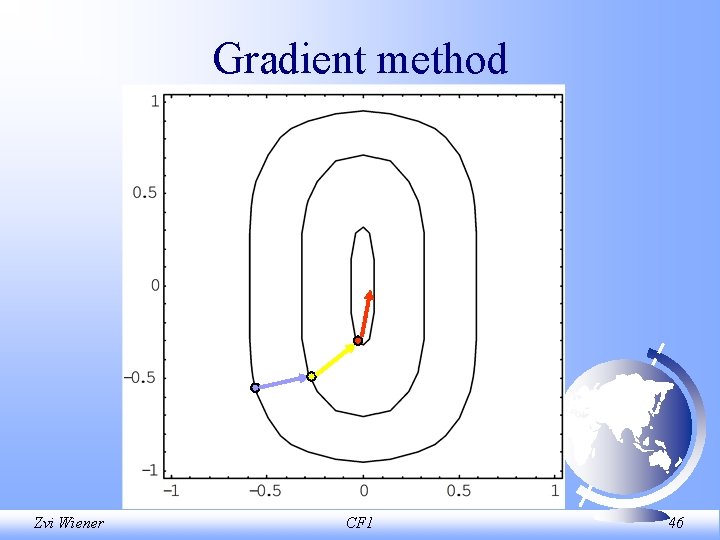
Gradient method Zvi Wiener CF 1 46

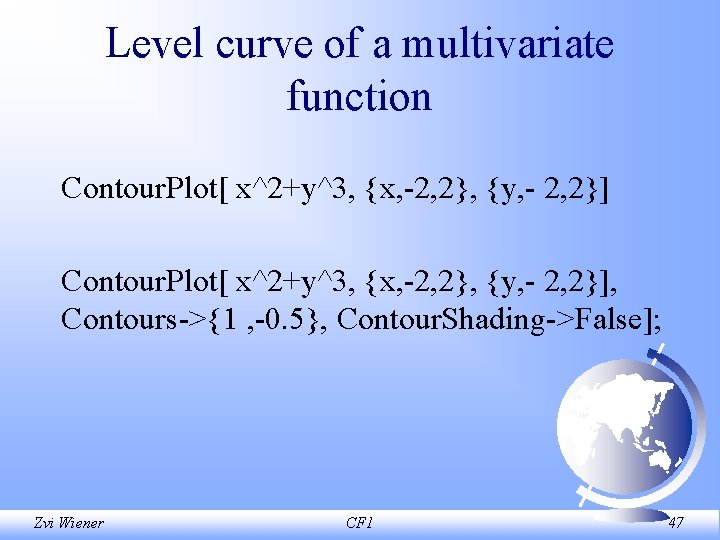
Level curve of a multivariate function Contour. Plot[ x^2+y^3, {x, 2, 2}, {y, 2, 2}], Contours >{1 , 0. 5}, Contour. Shading >False]; Zvi Wiener CF 1 47

Contour. Plot[ x^2+y^3, {x, 2, 2}, {y, 2, 2}] Zvi Wiener CF 1 48

Contour. Plot[ x^2+y^3, {x, 2, 2}, {y, 2, 2}], Contours >{1 , 0. 5}, Contour. Shading >False]; Zvi Wiener CF 1 49

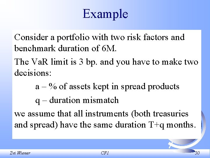
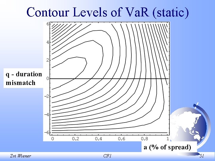
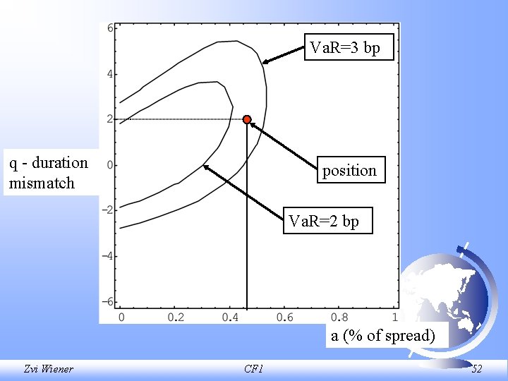
Example Consider a portfolio with two risk factors and benchmark duration of 6 M. The Va. R limit is 3 bp. and you have to make two decisions: a – % of assets kept in spread products q – duration mismatch we assume that all instruments (both treasuries and spread) have the same duration T+q months. Zvi Wiener CF 1 50

Contour Levels of Va. R (static) q - duration mismatch a (% of spread) Zvi Wiener CF 1 51

Va. R=3 bp q duration mismatch position Va. R=2 bp a (% of spread) Zvi Wiener CF 1 52

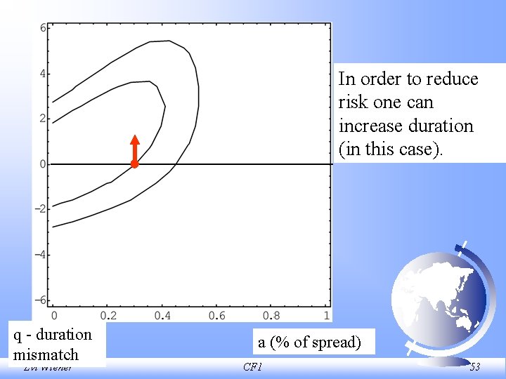
In order to reduce risk one can increase duration (in this case). q duration mismatch Zvi Wiener a (% of spread) CF 1 53

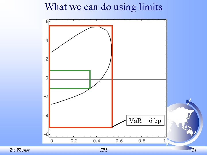
What we can do using limits Va. R = 6 bp Zvi Wiener CF 1 54

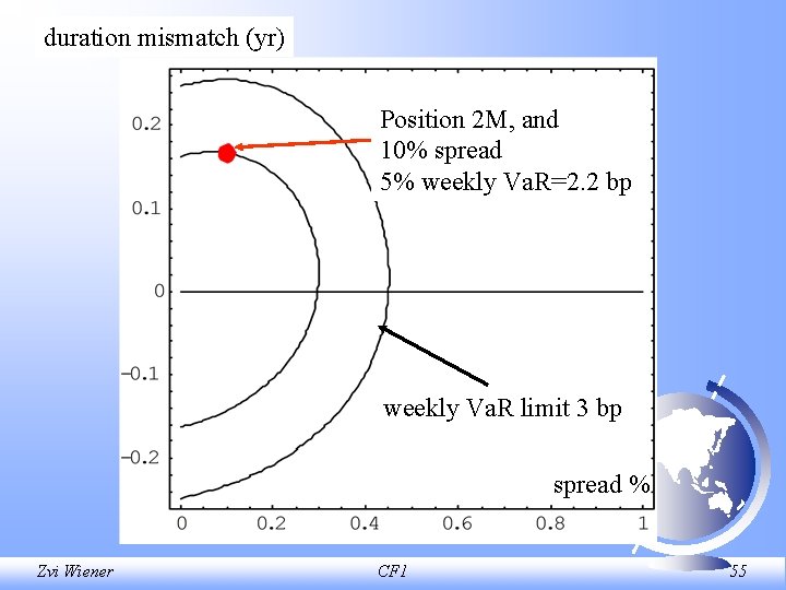
duration mismatch (yr) Position 2 M, and 10% spread 5% weekly Va. R=2. 2 bp weekly Va. R limit 3 bp spread % Zvi Wiener CF 1 55

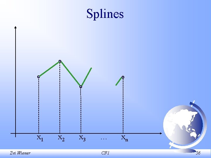
Splines x 1 Zvi Wiener x 2 x 3 … CF 1 xn 56

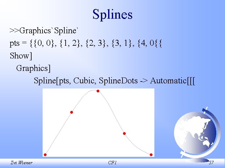
Splines >>Graphics`Spline` pts = {{0, 0}, {1, 2}, {2, 3}, {3, 1}, {4, 0{{ Show] Graphics] Spline[pts, Cubic, Spline. Dots > Automatic[[[ Zvi Wiener CF 1 57

Splines pts = Table[{i, i + i^2 + (Random[] 0. 5)}, {i, 0, 1, . 05}]; Show[Graphics[Spline[pts, Cubic, Spline. Dots >Automatic]]] Zvi Wiener CF 1 58

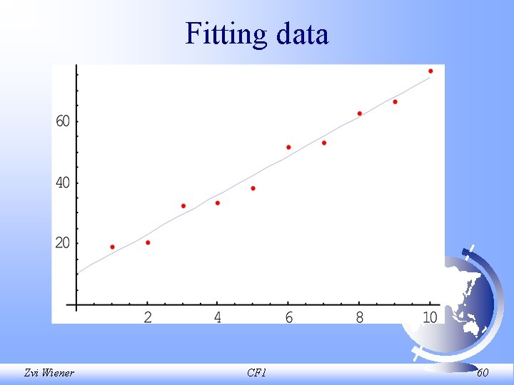
Fitting data = Table[7*x + 3 + 10*Random[], {x, 10}]; f[x_] : = Evaluate[Fit[data, {1, x}, x]] Needs["Graphics`"] Display. Together[ List. Plot[data, Plot. Style > {Absolute. Point. Size[3], RGBColor[1, 0, 0]}], Plot[f[x], {x, 0, 10}, Plot. Style > RGBColor[0, 0, 1]] ]; Zvi Wiener CF 1 59

Fitting data Zvi Wiener CF 1 60

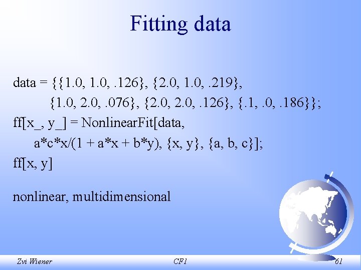
Fitting data = {{1. 0, . 126}, {2. 0, 1. 0, . 219}, {1. 0, 2. 0, . 076}, {2. 0, . 126}, {. 1, . 0, . 186}}; ff[x_, y_] = Nonlinear. Fit[data, a*c*x/(1 + a*x + b*y), {x, y}, {a, b, c}]; ff[x, y] nonlinear, multidimensional Zvi Wiener CF 1 61

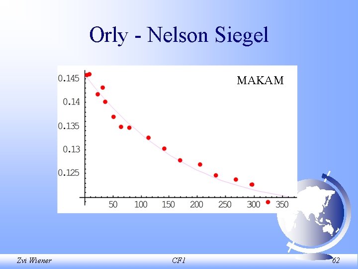
Orly Nelson Siegel MAKAM Zvi Wiener CF 1 62

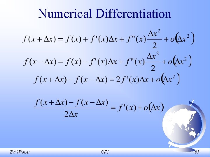
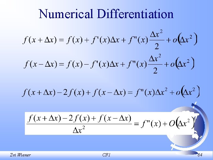
Numerical Differentiation Zvi Wiener CF 1 63

Numerical Differentiation Zvi Wiener CF 1 64

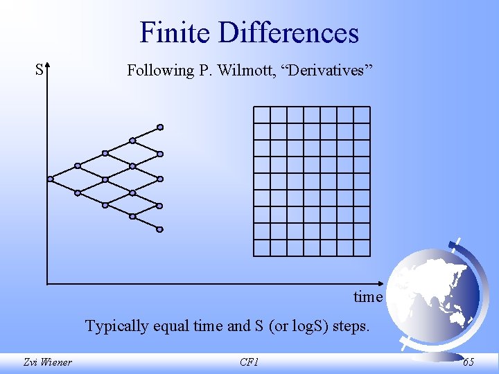
Finite Differences S Following P. Wilmott, “Derivatives” time Typically equal time and S (or log. S) steps. Zvi Wiener CF 1 65

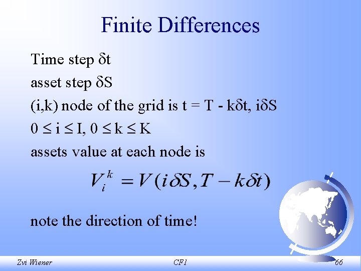
Finite Differences Time step t asset step S (i, k) node of the grid is t = T k t, i S 0 i I, 0 k K assets value at each node is note the direction of time! Zvi Wiener CF 1 66

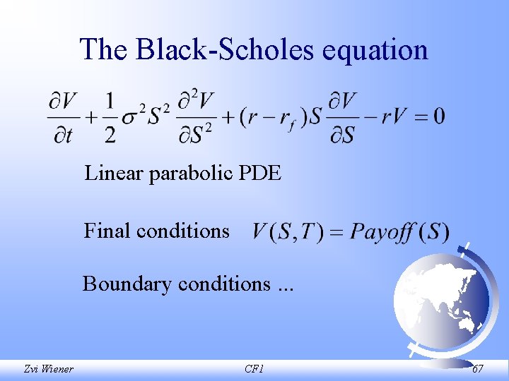
The Black Scholes equation Linear parabolic PDE Final conditions Boundary conditions. . . Zvi Wiener CF 1 67

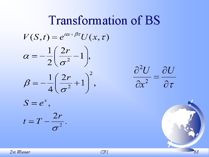
Transformation of BS Zvi Wiener CF 1 68

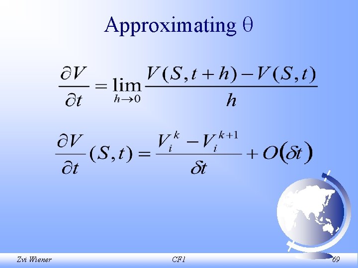
Approximating Zvi Wiener CF 1 69

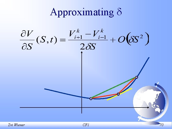
Approximating Zvi Wiener CF 1 70

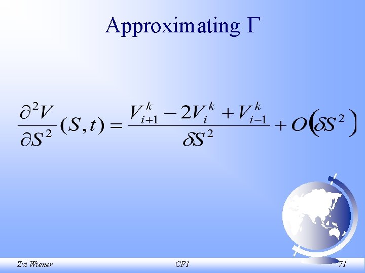
Approximating Zvi Wiener CF 1 71

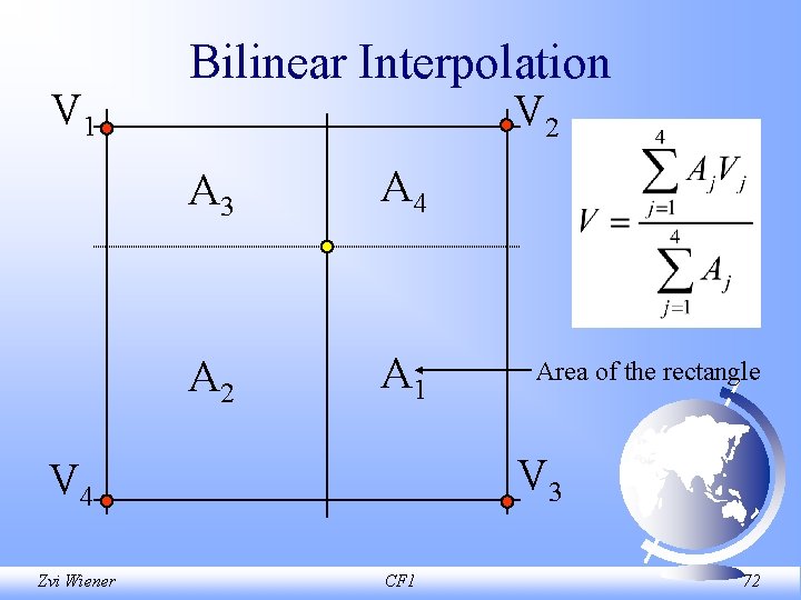
V 1 Bilinear Interpolation V 2 A 3 A 4 A 2 A 1 V 3 V 4 Zvi Wiener Area of the rectangle CF 1 72

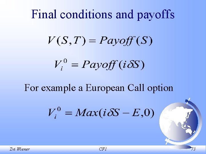
Final conditions and payoffs For example a European Call option Zvi Wiener CF 1 73

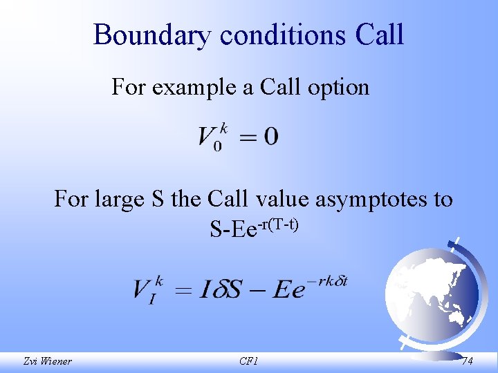
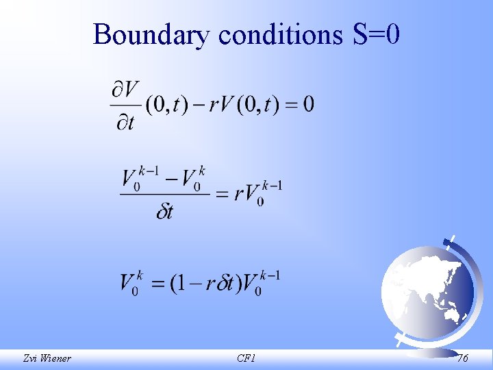
Boundary conditions Call For example a Call option For large S the Call value asymptotes to S Ee r(T t) Zvi Wiener CF 1 74

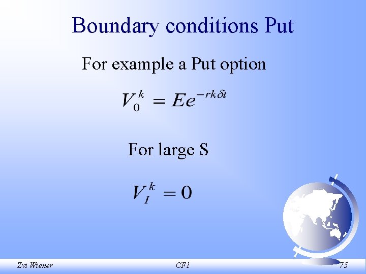
Boundary conditions Put For example a Put option For large S Zvi Wiener CF 1 75

Boundary conditions S=0 Zvi Wiener CF 1 76

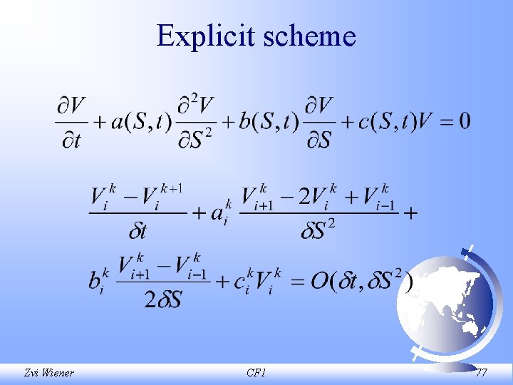
Explicit scheme Zvi Wiener CF 1 77

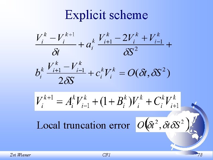
Explicit scheme Local truncation error Zvi Wiener CF 1 78

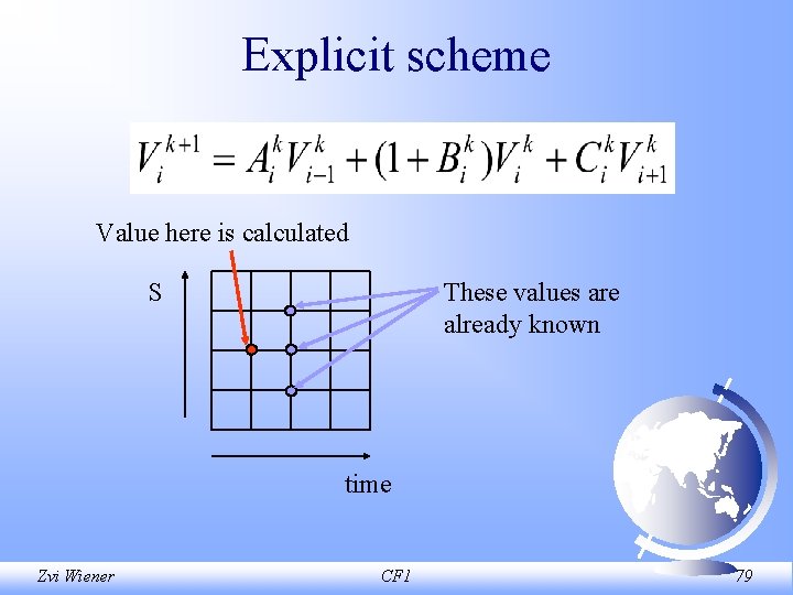
Explicit scheme Value here is calculated S These values are already known time Zvi Wiener CF 1 79

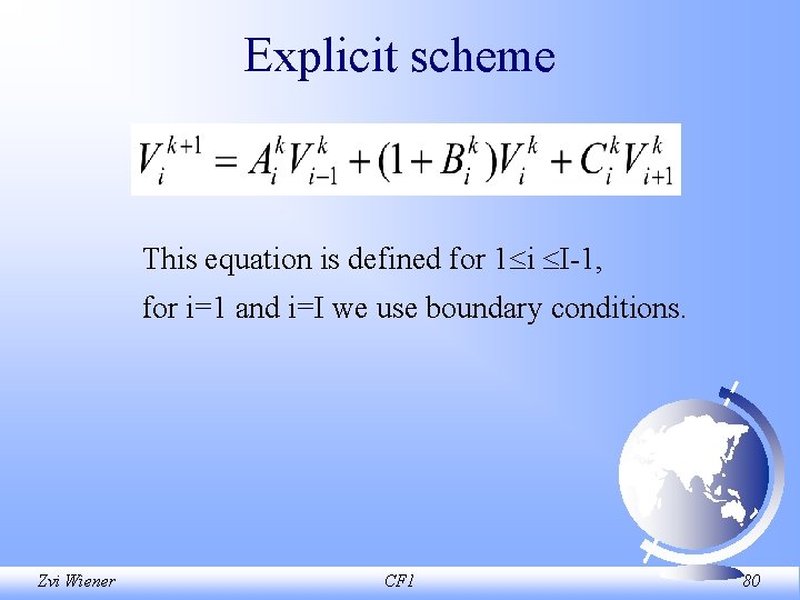
Explicit scheme This equation is defined for 1 i I 1, for i=1 and i=I we use boundary conditions. Zvi Wiener CF 1 80

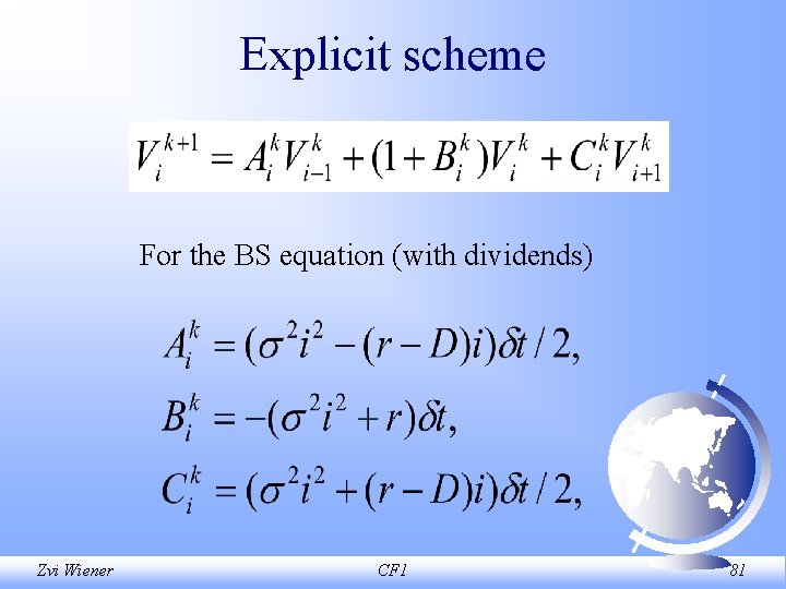
Explicit scheme For the BS equation (with dividends) Zvi Wiener CF 1 81

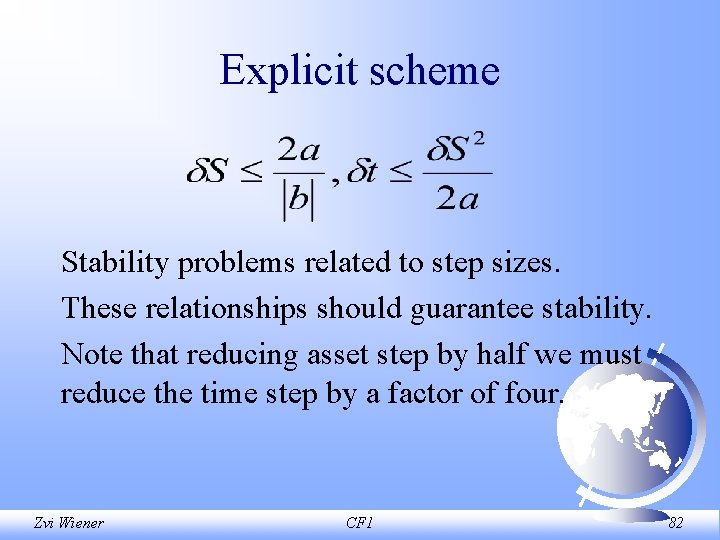
Explicit scheme Stability problems related to step sizes. These relationships should guarantee stability. Note that reducing asset step by half we must reduce the time step by a factor of four. Zvi Wiener CF 1 82

Explicit scheme Advantages easy to program, hard to make a mistake when unstable it is obvious coefficients can be S and t dependent Disadvantages there are restrictions on time step, which may cause slowness. Zvi Wiener CF 1 83

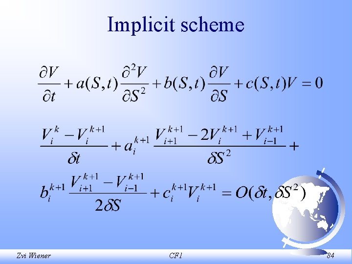
Implicit scheme Zvi Wiener CF 1 84

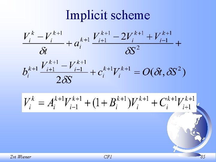
Implicit scheme Zvi Wiener CF 1 85

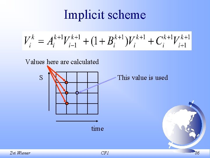
Implicit scheme Values here are calculated S This value is used time Zvi Wiener CF 1 86

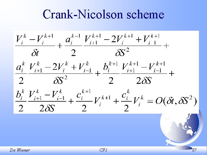
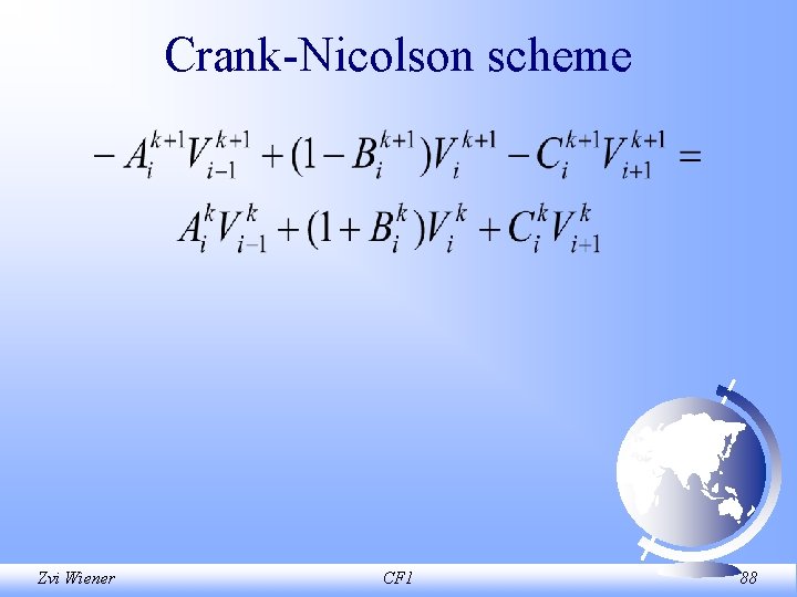
Crank Nicolson scheme Zvi Wiener CF 1 87

Crank Nicolson scheme Zvi Wiener CF 1 88

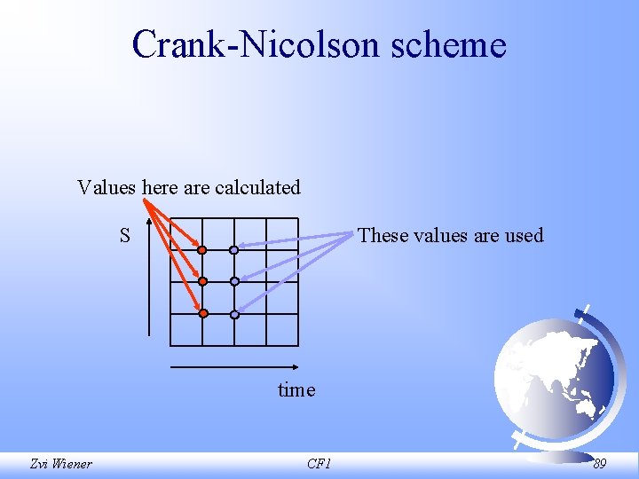
Crank Nicolson scheme Values here are calculated S These values are used time Zvi Wiener CF 1 89

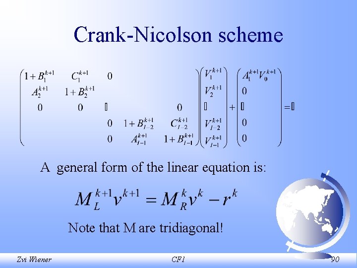
Crank Nicolson scheme A general form of the linear equation is: Note that M are tridiagonal! Zvi Wiener CF 1 90

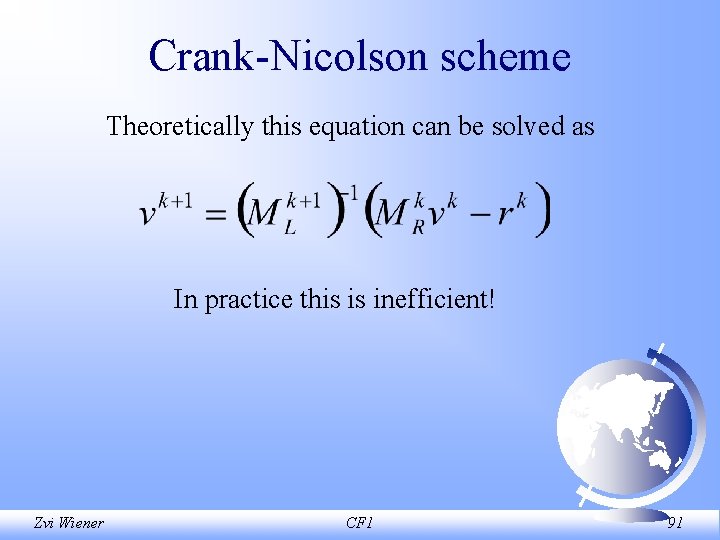
Crank Nicolson scheme Theoretically this equation can be solved as In practice this is inefficient! Zvi Wiener CF 1 91

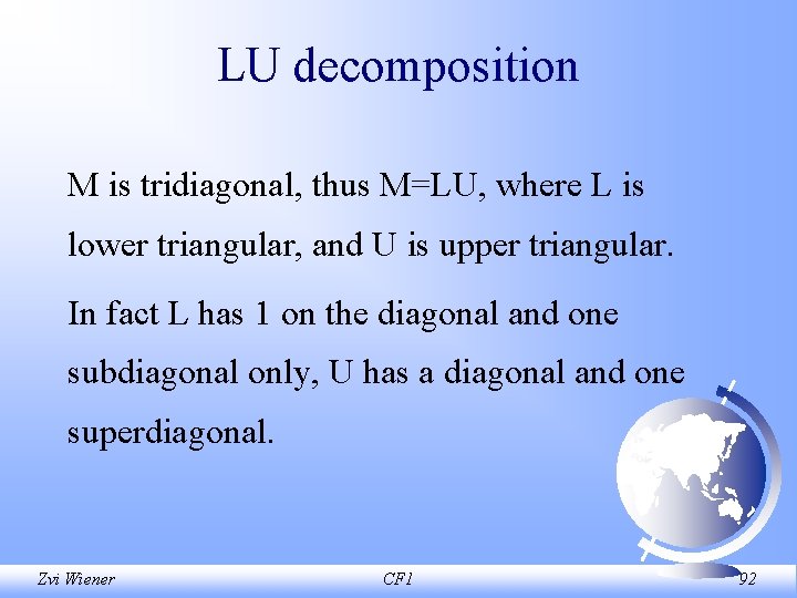
LU decomposition M is tridiagonal, thus M=LU, where L is lower triangular, and U is upper triangular. In fact L has 1 on the diagonal and one subdiagonal only, U has a diagonal and one superdiagonal. Zvi Wiener CF 1 92

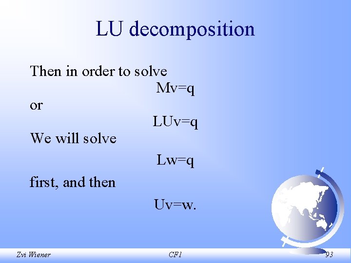
LU decomposition Then in order to solve Mv=q or LUv=q We will solve Lw=q first, and then Uv=w. Zvi Wiener CF 1 93

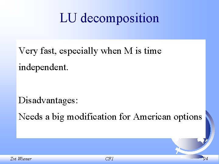
LU decomposition Very fast, especially when M is time independent. Disadvantages: Needs a big modification for American options Zvi Wiener CF 1 94

Other methods • SOR successive over relaxation • Douglas scheme • Three time level scheme • Alternating direction method • Richardson Extrapolation • Hopscotch method • Multigrid methods Zvi Wiener CF 1 95

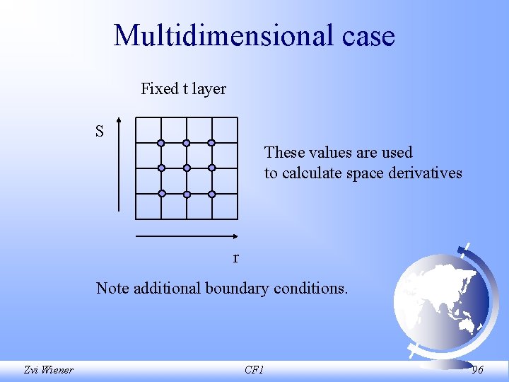
Multidimensional case Fixed t layer S These values are used to calculate space derivatives r Note additional boundary conditions. Zvi Wiener CF 1 96

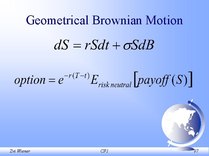
Geometrical Brownian Motion Zvi Wiener CF 1 97

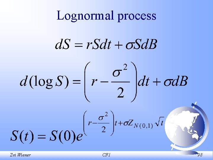
Lognormal process Zvi Wiener CF 1 98

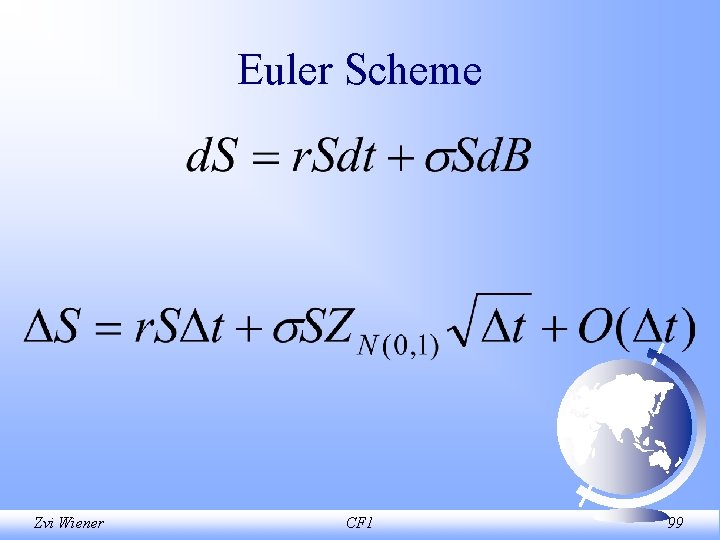
Euler Scheme Zvi Wiener CF 1 99

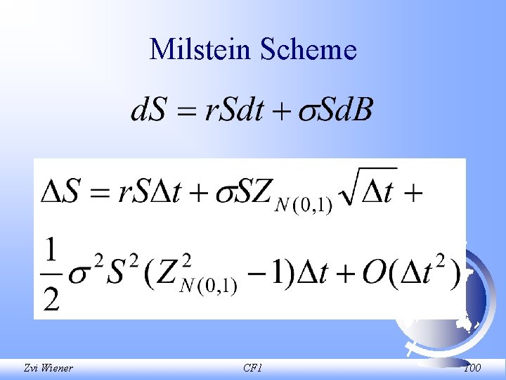
Milstein Scheme Zvi Wiener CF 1 100

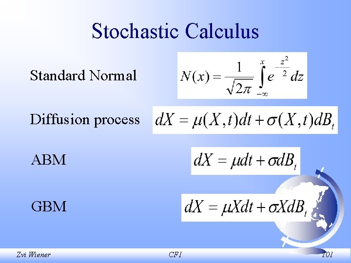
Stochastic Calculus Standard Normal Diffusion process ABM GBM Zvi Wiener CF 1 101

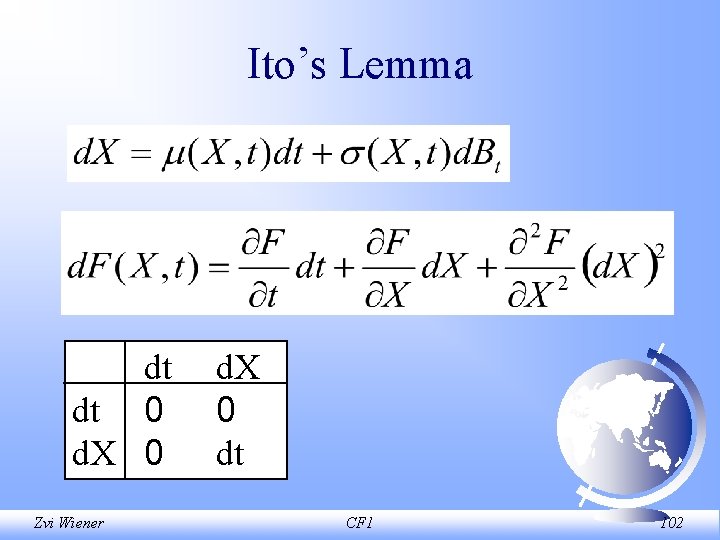
Ito’s Lemma dt dt 0 d. X 0 Zvi Wiener d. X 0 dt CF 1 102

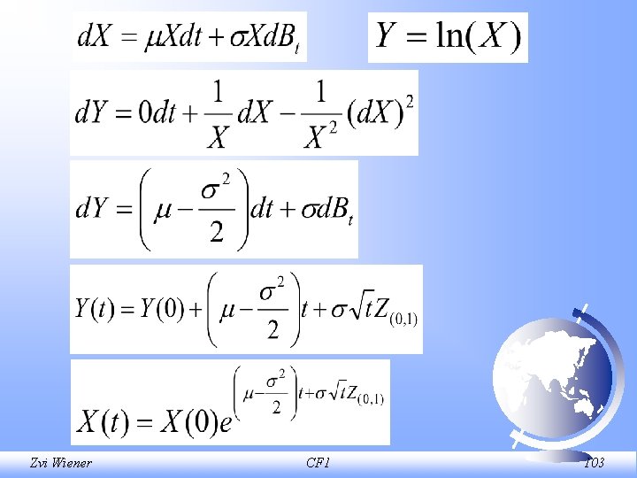
Zvi Wiener CF 1 103

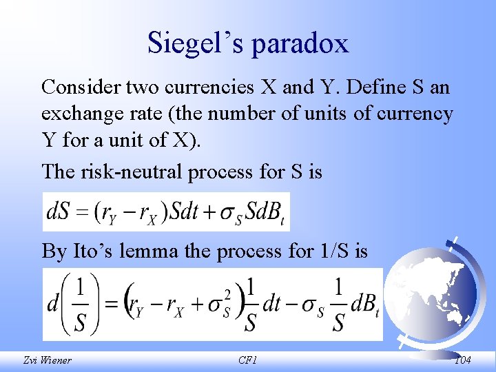
Siegel’s paradox Consider two currencies X and Y. Define S an exchange rate (the number of units of currency Y for a unit of X). The risk neutral process for S is By Ito’s lemma the process for 1/S is Zvi Wiener CF 1 104

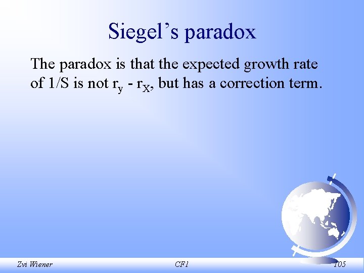
Siegel’s paradox The paradox is that the expected growth rate of 1/S is not ry r. X, but has a correction term. Zvi Wiener CF 1 105