Computational Finance Zvi Wiener 02 588 3049 http

Computational Finance Zvi Wiener 02 -588 -3049 http: //pluto. mscc. huji. ac. il/~mswiener/zvi. html CF-4 Bank Hapoalim Jun-2001

Plan 1. Monte Carlo Method 2. Variance Reduction Methods 3. Quasi Monte Carlo 4. Permuting QMC sequences 5. Dimension reduction 6. Financial Applications simple and exotic options American type prepayments Zvi Wiener CF 4 2

Monte Carlo Zvi Wiener CF 4 3

Monte Carlo Zvi Wiener CF 4 4

Monte Carlo Zvi Wiener CF 4 5

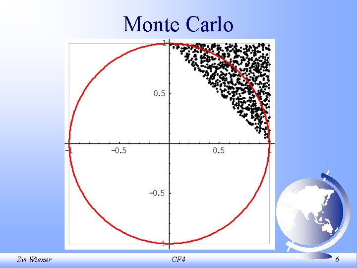
Monte Carlo Zvi Wiener CF 4 6

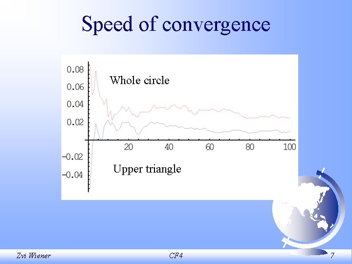
Speed of convergence Whole circle Upper triangle Zvi Wiener CF 4 7

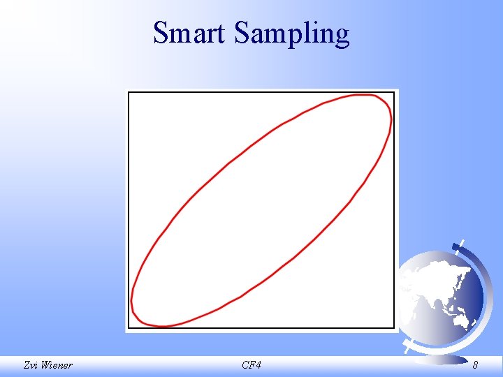
Smart Sampling Zvi Wiener CF 4 8

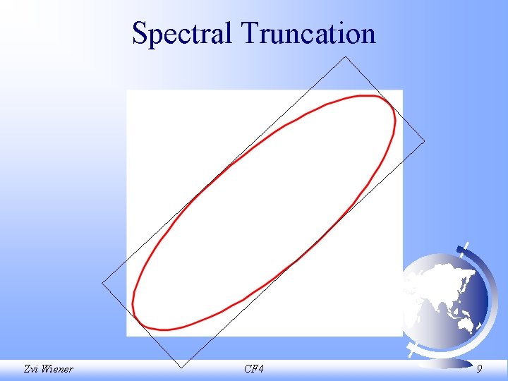
Spectral Truncation Zvi Wiener CF 4 9

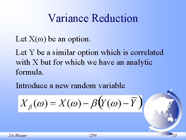
Variance Reduction Let X( ) be an option. Let Y be a similar option which is correlated with X but for which we have an analytic formula. Introduce a new random variable Zvi Wiener CF 4 10

Variance Reduction The variance of the new variable is If 2 cov[X, Y] > 2 var[Y] we have reduced the variance. Zvi Wiener CF 4 11

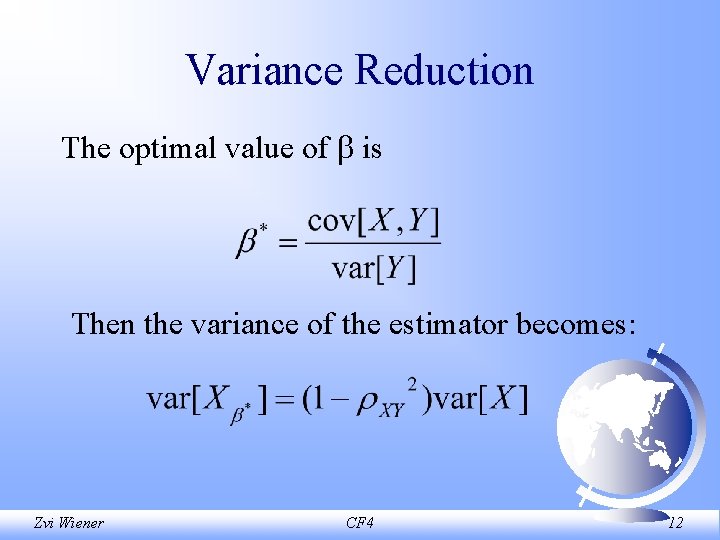
Variance Reduction The optimal value of is Then the variance of the estimator becomes: Zvi Wiener CF 4 12

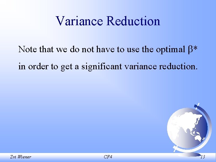
Variance Reduction Note that we do not have to use the optimal * in order to get a significant variance reduction. Zvi Wiener CF 4 13

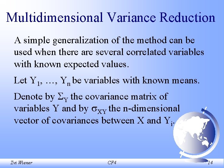
Multidimensional Variance Reduction A simple generalization of the method can be used when there are several correlated variables with known expected values. Let Y 1, …, Yn be variables with known means. Denote by Y the covariance matrix of variables Y and by XY the n-dimensional vector of covariances between X and Yi. Zvi Wiener CF 4 14

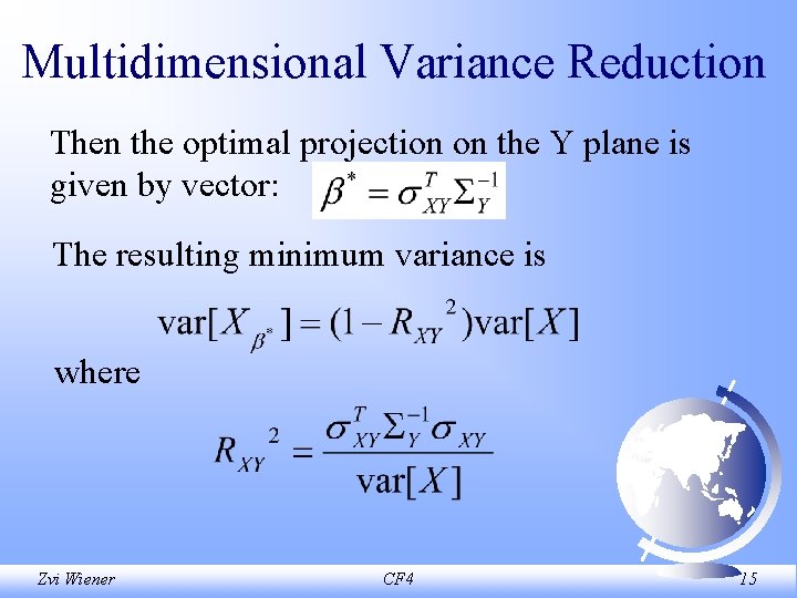
Multidimensional Variance Reduction Then the optimal projection on the Y plane is given by vector: The resulting minimum variance is where Zvi Wiener CF 4 15

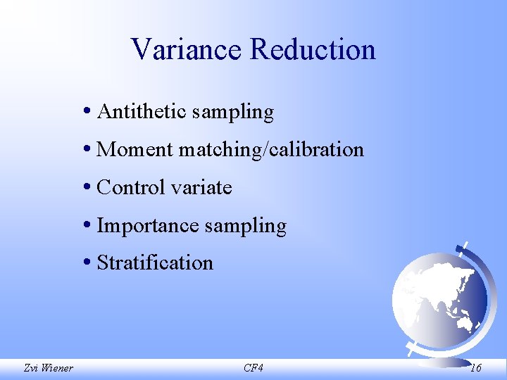
Variance Reduction • Antithetic sampling • Moment matching/calibration • Control variate • Importance sampling • Stratification Zvi Wiener CF 4 16

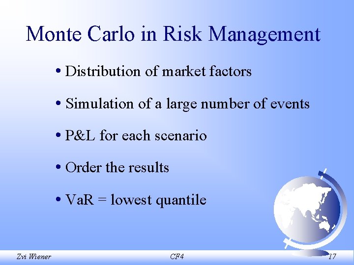
Monte Carlo in Risk Management • Distribution of market factors • Simulation of a large number of events • P&L for each scenario • Order the results • Va. R = lowest quantile Zvi Wiener CF 4 17

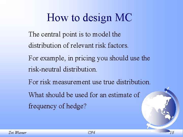
How to design MC The central point is to model the distribution of relevant risk factors. For example, in pricing you should use the risk-neutral distribution. For risk measurement use true distribution. What should be used for an estimate of frequency of hedge? Zvi Wiener CF 4 18

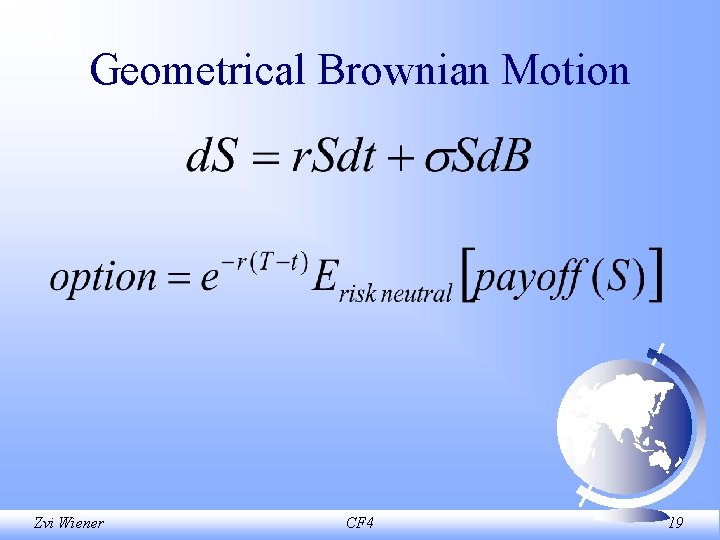
Geometrical Brownian Motion Zvi Wiener CF 4 19

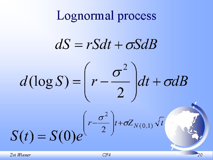
Lognormal process Zvi Wiener CF 4 20

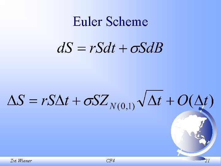
Euler Scheme Zvi Wiener CF 4 21

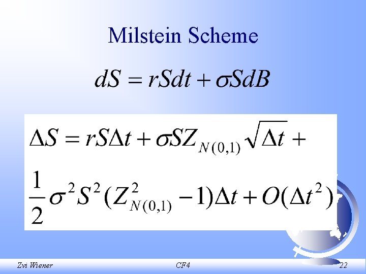
Milstein Scheme Zvi Wiener CF 4 22

MC for simple options Needs["Statistics`Normal. Distribution`"] Clear[MCEuropean, MCEuropean. Call, MCEuropean. Put] nor[mu_, sig_]: =Random[Normal. Distribution[mu, sig]]; Zvi Wiener CF 4 23

MC for simple options MCEuropean[s_, T_, r_, _, n_, exercise_Function]: = Module[{m = N[Log[s]+(r - 0. 5 2)*T], sg=N[ Sqrt[T] ], tbl}, tbl= Table[nor[m, sg], {i, n}]; Exp[-r*T]*Map[exercise, Exp[Join[tbl, 2*m - tbl]]]// {Mean[#], Standard. Error. Of. Sample. Mean[#]}& ] Zvi Wiener CF 4 24

MC for simple options MCEuropean. Call[s_, x_, T_, r_, _, n_]: = MCEuropean[s, T, r, , n, Max[#-x, 0]&] MCEuropean. Put[s_, x_, T_, r_, _, n_]: = MCEuropean[s, T, r, , n, Max[x-#, 0]&] Zvi Wiener CF 4 25

MC for path dependent options Random. Walk[n_Integer=: [ Fold. List[Plus, 0, Table[Random[] - 1/2, {n; [[{ List. Plot[ Random. Walk[500], Plot. Joined -> True; [ Zvi Wiener CF 4 26

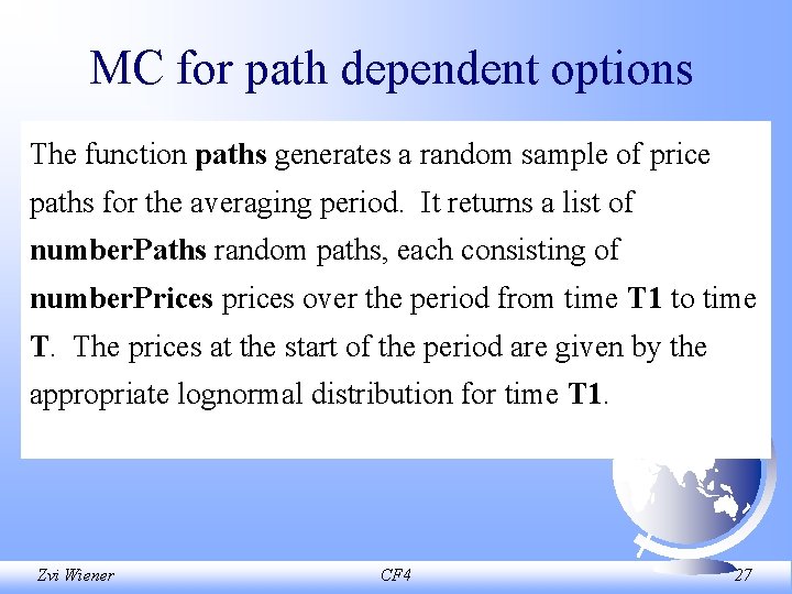
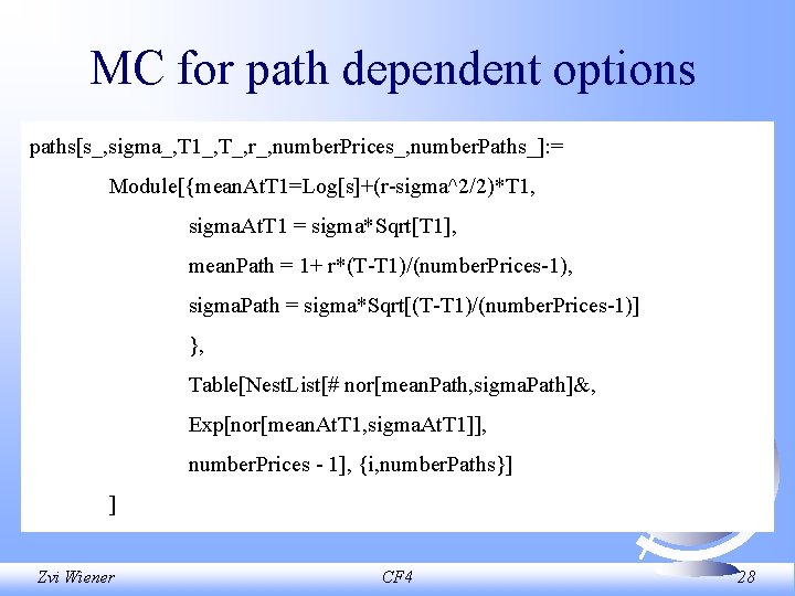
MC for path dependent options The function paths generates a random sample of price paths for the averaging period. It returns a list of number. Paths random paths, each consisting of number. Prices prices over the period from time T 1 to time T. The prices at the start of the period are given by the appropriate lognormal distribution for time T 1. Zvi Wiener CF 4 27

MC for path dependent options paths[s_, sigma_, T 1_, T_, r_, number. Prices_, number. Paths_]: = Module[{mean. At. T 1=Log[s]+(r-sigma^2/2)*T 1, sigma. At. T 1 = sigma*Sqrt[T 1], mean. Path = 1+ r*(T-T 1)/(number. Prices-1), sigma. Path = sigma*Sqrt[(T-T 1)/(number. Prices-1)] }, Table[Nest. List[# nor[mean. Path, sigma. Path]&, Exp[nor[mean. At. T 1, sigma. At. T 1]], number. Prices - 1], {i, number. Paths}] ] Zvi Wiener CF 4 28

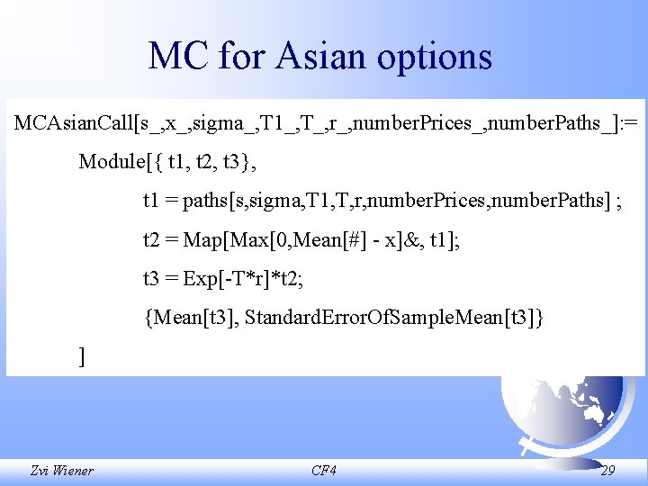
MC for Asian options MCAsian. Call[s_, x_, sigma_, T 1_, T_, r_, number. Prices_, number. Paths_]: = Module[{ t 1, t 2, t 3}, t 1 = paths[s, sigma, T 1, T, r, number. Prices, number. Paths] ; t 2 = Map[Max[0, Mean[#] - x]&, t 1]; t 3 = Exp[-T*r]*t 2; {Mean[t 3], Standard. Error. Of. Sample. Mean[t 3]} ] Zvi Wiener CF 4 29

Quasi Monte Carlo • Van der Corput • Halton • Haber • Sobol • Faure • Niederreiter • Permutations • Nets Zvi Wiener CF 4 30

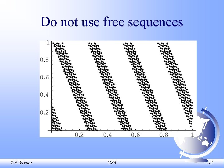
Quasi Monte Carlo Are efficient in low (1 -2) dimensions. Sobol sequences can be used for small dimensions as well. As an alternative one can create a fixed set of well-distributed paths. Zvi Wiener CF 4 31

Do not use free sequences Zvi Wiener CF 4 32

Other MC applications • Pricing • Optimal hedging • Impact of dividends • Bounds on a basket • Prepayments • Tranches of MBS Zvi Wiener CF 4 33

Other MC related topics Use of analytical approximations Richardson extrapolation Ratchets example American properties Bundling Modeling Fat tails Zvi Wiener CF 4 34

Value of Value-at-Risk Zvi Wiener The Hebrew University of Jerusalem mswiener@mscc. huji. ac. il CF-4 Bank Hapoalim Jun-2001

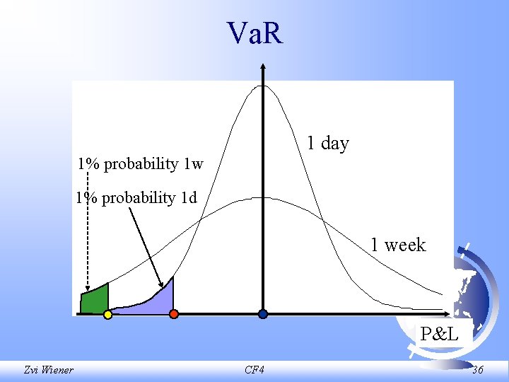
Va. R 1 day 1% probability 1 w 1% probability 1 d 1 week P&L Zvi Wiener CF 4 36

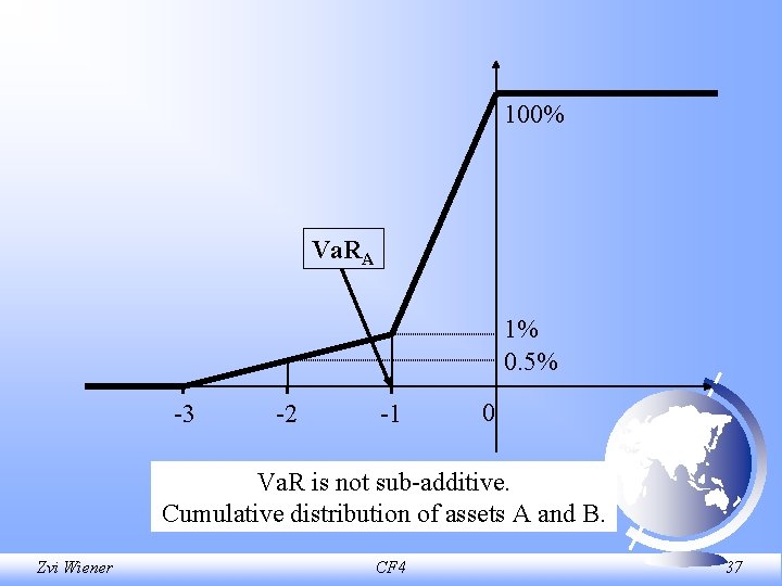
100% Va. RA 1% 0. 5% -3 -2 -1 0 Va. R is not sub-additive. Cumulative distribution of assets A and B. Zvi Wiener CF 4 37

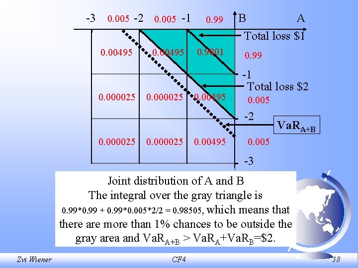
-3 0. 005 -2 0. 005 -1 0. 99 B A Total loss $1 0. 00495 0. 000025 0. 9801 0. 00495 0. 99 -1 Total loss $2 0. 005 -2 0. 000025 0. 00495 Va. RA+B 0. 005 -3 Joint distribution of A and B The integral over the gray triangle is 0. 99*0. 99 + 0. 99*0. 005*2/2 = 0. 98505, which means that there are more than 1% chances to be outside the gray area and Va. RA+B > Va. RA+Va. RB=$2. Zvi Wiener CF 4 38

Model • Bank’s choice of an optimal system • Depends on the available capital • Current and potential capital needs • Queuing model as a base Zvi Wiener CF 4 39

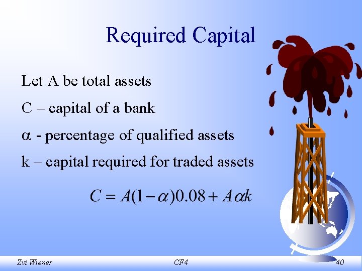
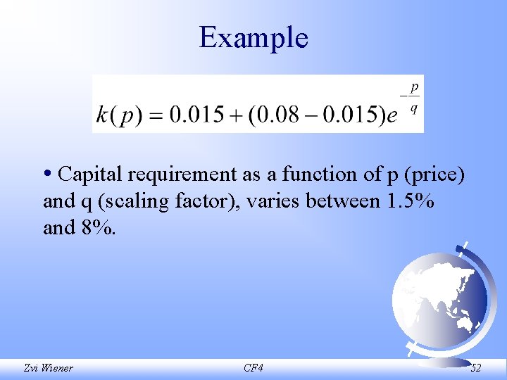
Required Capital Let A be total assets C – capital of a bank - percentage of qualified assets k – capital required for traded assets Zvi Wiener CF 4 40

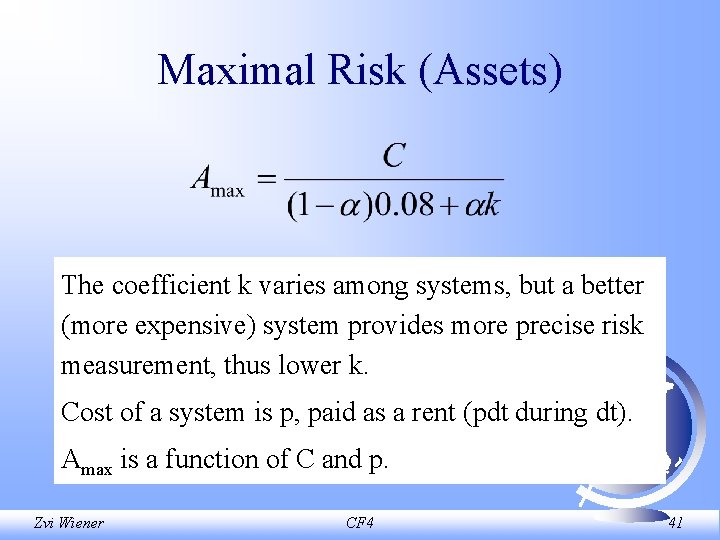
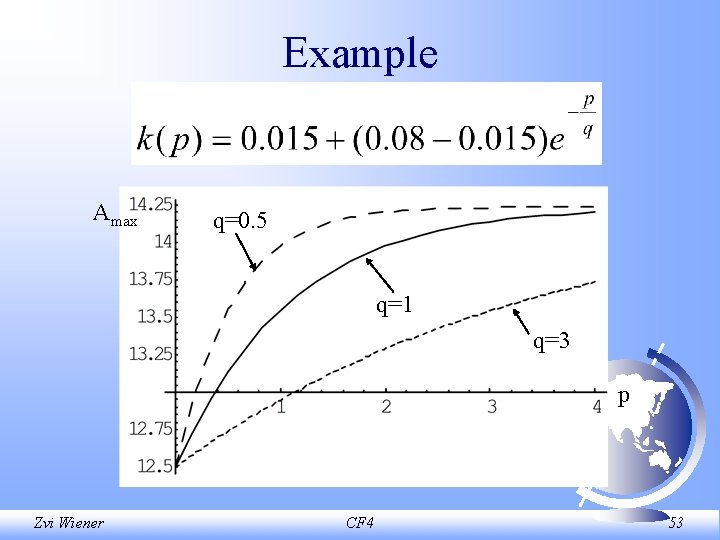
Maximal Risk (Assets) The coefficient k varies among systems, but a better (more expensive) system provides more precise risk measurement, thus lower k. Cost of a system is p, paid as a rent (pdt during dt). Amax is a function of C and p. Zvi Wiener CF 4 41

Risky Projects Deposits arrive and are withdrawn randomly. All deposits are of the same size. Invested according to bank’s policy. Can not be used if capital requirements are not satisfied. Zvi Wiener CF 4 42

Arrival of Risky Projects We assume that risky projects arrive randomly (as a Poisson process with density ). This means that there is a probability dt that during dt one new project arrives. Zvi Wiener CF 4 43

Arrival of Risky Projects A new project is undertaken if the bank has enough capital (according to the existing risk measuring system). We assume that one can NOT raise capital or change systems quickly. Zvi Wiener CF 4 44

Termination of Risky Projects We assume that each risky project disappears randomly (as a Poisson process with density ). Zvi Wiener CF 4 45

Termination of Risky Projects We assume that each risky project disappears randomly (as a Poisson process with density ). This means that there is a probability n dt that during dt one out of n existing projects terminates. With probability (1 -n dt) all existing projects will be active after dt. Zvi Wiener CF 4 46

Profit We assume that each existing risky project gives a profit of dt during dt. Thus when there are n active projects the bank has instantaneous profit ( n-p)dt. Zvi Wiener CF 4 47

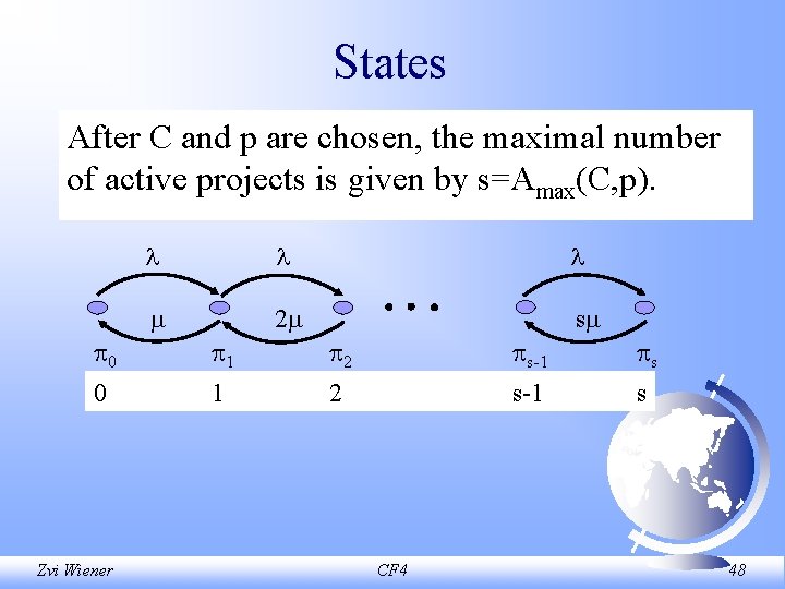
States After C and p are chosen, the maximal number of active projects is given by s=Amax(C, p). 2 s 0 1 2 s-1 s 0 1 2 s-1 s Zvi Wiener CF 4 48

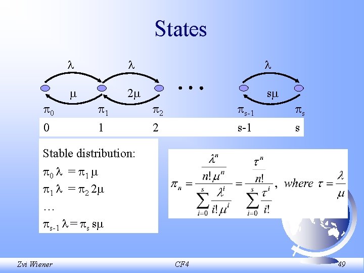
States 2 s 0 1 2 s-1 s 0 1 2 s-1 s Stable distribution: 0 = 1 1 = 2 2 … s-1 = s s Zvi Wiener CF 4 49

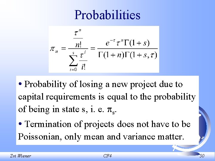
Probabilities • Probability of losing a new project due to capital requirements is equal to the probability of being in state s, i. e. s. • Termination of projects does not have to be Poissonian, only mean and variance matter. Zvi Wiener CF 4 50

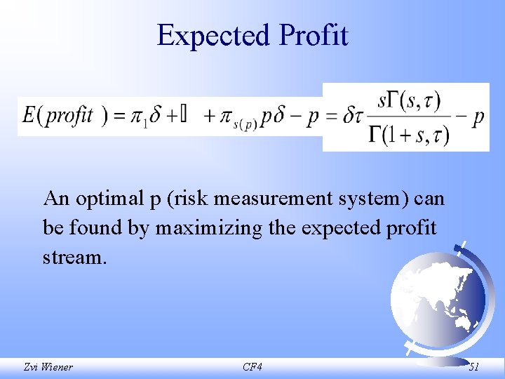
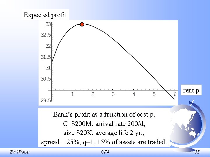
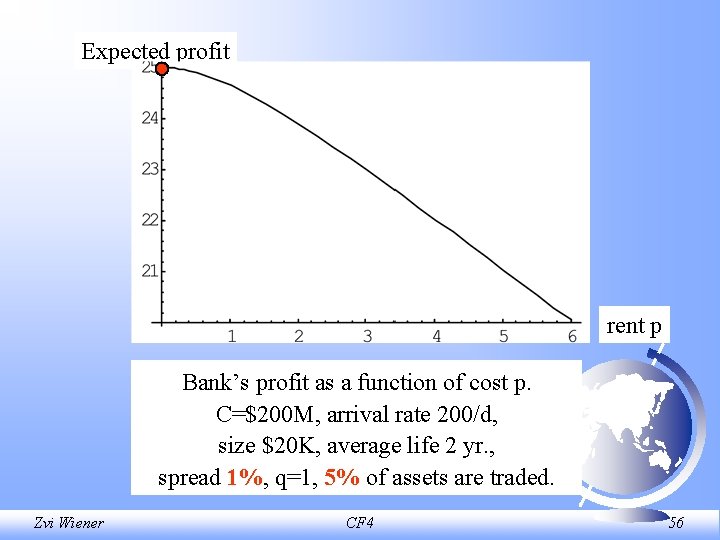
Expected Profit An optimal p (risk measurement system) can be found by maximizing the expected profit stream. Zvi Wiener CF 4 51

Example • Capital requirement as a function of p (price) and q (scaling factor), varies between 1. 5% and 8%. Zvi Wiener CF 4 52

Example Amax q=0. 5 q=1 q=3 p Zvi Wiener CF 4 53

Example of a bank • Capital $200 M • Average project is $20 K • On average 200 new projects arrive each day • Average life of a project is 2 years • 15% of assets are traded and q=1 • spread =1. 25% Zvi Wiener CF 4 54

Expected profit rent p Bank’s profit as a function of cost p. C=$200 M, arrival rate 200/d, size $20 K, average life 2 yr. , spread 1. 25%, q=1, 15% of assets are traded. Zvi Wiener CF 4 55

Expected profit rent p Bank’s profit as a function of cost p. C=$200 M, arrival rate 200/d, size $20 K, average life 2 yr. , spread 1%, q=1, 5% of assets are traded. Zvi Wiener CF 4 56

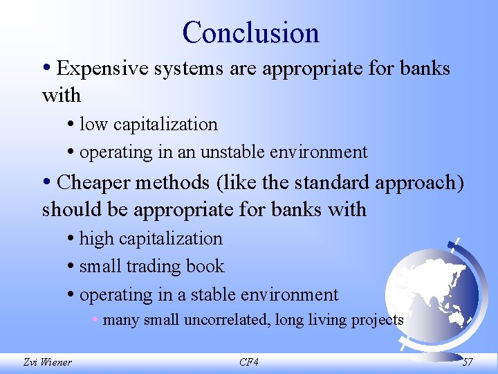
Conclusion • Expensive systems are appropriate for banks with • low capitalization • operating in an unstable environment • Cheaper methods (like the standard approach) should be appropriate for banks with • high capitalization • small trading book • operating in a stable environment • many small uncorrelated, long living projects Zvi Wiener CF 4 57

A simple intuitive and flexible model of optimal choice of risk measuring method. Zvi Wiener CF 4 58