computational aggregation scott e page university of michigan

computational aggregation scott e page university of michigan santa fe institute

Evolving Interpretations and the Possibility of Collective Wisdom Jenna Bednar Lu Hong Ken Kollman PJ Lamberson Scott Page Maria Riolo Nathan Seegert

Outline The Wisdom of Crowds - anecdote - undergraduate - graduate Generated vs Interpreted Signals - foundations - statistical properties

UCSC

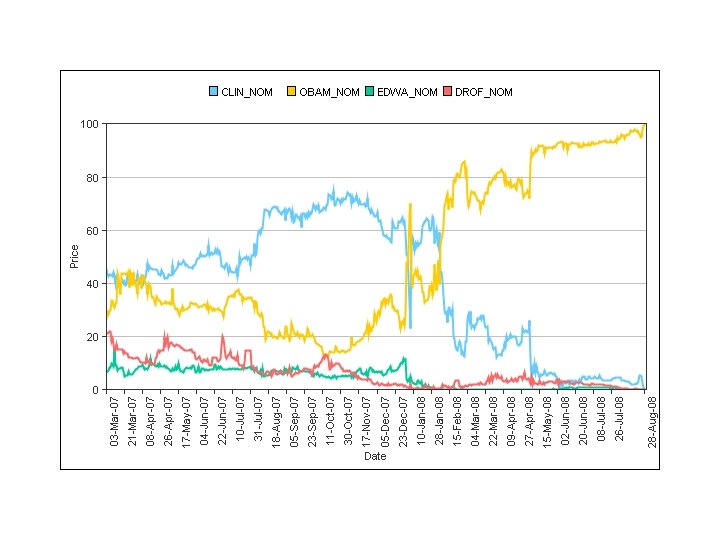
Iowa Electronic Markets IEM Prices Obama 0. 535 Mc. Cain 0. 464 Final Gallup Poll Obama 0. 55 Mc. Cain 0. 44 Actual Outcome Obama 0. 531 Mc. Cain 0. 469 Oxford 5 -1 - 07

Interpreted vs Generated Signal: truth plus a disturbance or interference Interpreted Signal: prediction from a model

Generated Signal noise Outcome Signal

UCSC

L- L+

L

Generated Signals Independent Common correlation Common bias Produced in any number by some generating process UCSC

Voting vs Markets Voting: all models get equal weight Markets: models can get differential weight

Signals as Predictions Outcome in N individuals indexed by i Signal received by i: si Vector of signals: s = (s 1, s 2, … sn ) f(si si | ) = distribution of signals si conditional on . The signals are often assumed to be independent

Measures Squared Error for individual i: Sq. E(si) = (si - )2 Average Squared Error: Sq. E(s) = Collective Prediction: c = Collective Squared Error: Sq. E(c) = (c - )2 Predictive Diversity: PDiv(s) =

Diversity Prediction Theorem Sq. E(c) = Sq. E(s) - PDiv(s)

Crowd Error = Average Error - Diversity 0. 6 = 2, 956. 0 - 2955. 4

Signals as Random Variables Mean of i’s signal: i( ) Bias of i’s signal: bi = ( i( ) - ) Variance of i’s signal: vi =E[( i( ) - )]2 Average Bias B = Average Variance V = Average Covariance C =

Bias Variance Decomposition Ensemble Learning Theory E[Sq. E(c)] =

Resolving the Paradox Diversity Prediction Theorem: Predictive Diversity is realized diversity, which improves accuracy. Bias Variance Decomposition: Variance corresponds to noisier signals, which reduces accuracy. Negative covariance implies diverse realized diversity and improves expected accuracy of collective predictions.

Large Population Accuracy If the signals are independent, unbiased, and with bounded variance, then as n approaches infinity the crowd’s error goes to zero E[Sq. E(c)] =

Interpretive Signal model Attributes Prediction

Interpretations Reality consists of many variables or attributes. People cannot include them all. Therefore, we consider only some attributes or lump things together into categories. (Reed, Rosch, Mullinathun, Jackson and Fryer, Collins)

West Virginia Congressional District 1 District 2 District 3

West Virginia Slaw available on reque Slaw standard on hot d Slaw not available No data available

Interpretations: Pile Sort Place the following food items in piles Broccoli Fresh Salmon Spam Niman Pork Carrots Arugula Ahi Tuna Sea Bass Canned Beets Fennel Canned Posole Canned Salmon

BOBO Sort Veggie Organic Broccoli Arugula Carrots Fennel Fresh Salmon Sea Bass Niman Pork Ahi Tuna Canned Beets Spam Canned Salmon Canned Posole

Airstream Sort Veggie Meat/Fish Weird? Broccoli Fennel Carrots Canned Beets Fresh Salmon Canned Posole Spam Sea Bass Niman Pork Arugula Canned Salmon Ahi Tuna

Interpretive Signal model Attributes Prediction

Interpretive Signal Example Charisma Experience H MH ML L H G G G B MH G G G B G ML G B B B L B G B B

Experience Interpretation 75 % Correct H G G G B MH G G G B ML G B B L B G B B B

Interpreted Signals Statistical assumptions depend on diversity and sophistication. Independent? Positive correlation and bias result from similar models Amount of potential diversity and sophistication depend on complexity and dimensionality of outcome function

Binary Interpreted Signals Model Set of objects |X|=N Set of outcomes S = {G, B} Interpretation: Ij = {mj, 1, mj, 2…mj, nj} is a partition of X P(mj, i) = probability mj, i arises

Independent Interpretations P(mji and mkl) = P(mji)P(mkl) Probability j says “i” and k say “el”equals the product of the probability that j says “i” times the probability k says “el”.

Why Independence? We’re interested in independent interpretations because that’s the best people or agents could do in the binary setting. It’s the most diverse two predictions could be. Captures a world in which agents or people look at distinct pieces of information.

Claim: Independent, informative interpreted signals that predict good and bad outcomes with equal likelihood must be negatively correlated in their correctness.

Proof g g b Prob row correct: Prob column correct: Prob both correct: b G=X B = 1 -X G=Y B = 1 -Y G=Z B = 1 -Z G=W B = 1 -W (X+Y+2 -(W+Z))/4 (X+Z+2 -(W+Y))/4 (X+1 -W)/4 (X+Y+2 -(W+Z))(X+Z+2 -(W+Y)) - 4(X+1 -W) = (X-W)2 - (Y-Z)2 > 0

Claim: Independent, informative interpreted signals that predict good and bad outcomes with equal likelihood that are correct with probability p exhibit negative correlation equal to Note: p is bounded above by 0. 75

The following assumptions are inconsistent with independent interpreted signals States = {G, B} equally likely Signals = {g, b} conditionally independent on the state.

Independent Interpreted Signals Interpreted signal: sj(mji) prediction by j given in set I Interpreted signals are independent iff sj(mji) and sk(mkl) are independent random variables.

Claim: Any outcome function that produces conditionally independent interpreted signals is isomorphic to this example.

! Claim: For signals based on independent interpretations, the difficulty of the outcome function does not alter correlation other than through the accuracy of the interpreted signals

Proof g g b b

Proof g b Probability that each is correct and that both are correct is unchanged

Interpretive Signal Example Charisma Experience H MH ML L H G G G B MH G G G B G ML G B B B L B G B B

Experience Interpretation 75 % Correct H G G G B MH G G G B ML G B B L B G B B B

Charisma Interpretation 75% Correct H MH ML L G G G B B G B B

Balanced Interpretation 75% Correct G B G G B Extreme on one measure. Moderate on the other G B G G B B

Voting Outcome H MH ML L H GGB GGG GBG BGB MH GGG GGB GBB G GBG ML BGG BBB BBG L BGB BGG BBB

Reality H MH ML L H G G G B MH G G G B G ML G B B B L B G B B

Recall Interpretation Ii = (mi 1, mi 2, …mik) partition of X Predictive Model Mi: X into {0, 1} s. t. if x, y in mij then Mi(x) = Mi(y)

Assumptions A 1 Common prior with full support A 2 State Relevance: Both predictions occur with positive probability A 3 Monotonicity : Let Pi(a | b) = Pi(outcome = a | i predicts b) Pi(1 | 1) > Pi(0 | 1) Pi(1 | 0) Pi(0 | 0)

Collective Measurability: The outcome function F is measurable with respect to (Mi) i N, the smallest sigma field such that all Mi are measurable. Proposition: F satisfies collective measurability if and only if F(x) = G(M 1(x)…Mn (x)) for all x in X

Agent 1 Outcome Function Agent 2

Agent 1 Outcome Function Agent 2

Threshold Separable Additivity: Given F, {Mi} i N, and G: {0, 1}N into {0, 1}, there exists an integer k and a set of functions hi : {0, 1} into {0, 1}, such that G(M 1(x)…Mn (x)) = 1 if and only if ∑ hi (Mi(x)) > k N. B. This does not mean that the function is linear in the models, only that it can be expressed this way!

Theorem: A classification problem can be solved by a threshold voting mechanism if and only if it satisfies collective measurability and threshold separable additivity with respect to the agents’ models.

Example 1 State (x 1, x 2 , x 3 , x 4 , x 5 , x 6 , x 7 , x 8 , x 9) xi in {0, 1} Outcome Function F(x 1, x 2 , x 3 , x 4 , x 5 , x 6 , x 7 , x 8 , x 9) = 1 iff 4 < ∑ x. I Interpretations I 1 = (x 1, #, #, …, #) I 2 = (#, x 2, #…, #) I 9 = (#, #, …, #, x 9)

Example 1 State (x 1, x 2 , x 3 , x 4 , x 5 , x 6 , x 7 , x 8 , x 9) xi in {0, 1} Outcome Function F(x 1, x 2 , x 3 , x 4 , x 5 , x 6 , x 7 , x 8 , x 9) = 1 iff 4 < ∑ x. I Interpretations I 1 = (x 1, #, #, …, #) I 2 = (#, x 2, #…, #) I 9 = (#, #, …, #, x 9) Voting Rule M(xi) = xi Proof: F(x 1, …, x 9 ) = ∑ M(x. I)

Example 2 State (x 1, x 2 , x 3 , x 4 , x 5 , x 6 , x 7 , x 8 , x 9) xi in {0, 1, 2} Outcome Function F(x 1, x 2 , x 3 , x 4 , x 5 , x 6 , x 7 , x 8 , x 9) = 1 iff 8 < ∑ x. I Interpretations I 1 = (x 1, x 2, x 3, . . , #) I 2 = (#, x 2, x 3, x 4, . . #) I 9 = (x 1, x 2, #, . . x 9)

Collective Measurability Outcome Function F(x 1, x 2 , x 3 , x 4 , x 5 , x 6 , x 7 , x 8 , x 9) = 1 iff 8 < ∑ x. I Interpretations I 1 = (x 1, x 2, x 3, #, …, #) I 2 = (#, x 2, x 3, x 4, #…, #) I 9 = (x 1, x 2, #, …, #, x 9) The smallest sigma field such that the interpretations are measurable is (x 1, x 2 , x 3 , x 4 , x 5 , x 6 , x 7 , x 8 , x 9) so collective measurability is satisfied.

Threshold Separable Additivity Voting Rule: M(xi, xi+1, xi+2) = 1 iff xi+1+xi+2 > 2 Counterexample 1: State = (0, 2, 1, 1, 2, 0, 0, 0) Outcome = 0 Votes: (Y, Y, N, N, N) Counterexample 2: State = (2, 2, 0, 0, 1, 0, 0 2, 2) Outcome = 1 Votes: (Y, N, N, N, Y, Y, Y)

Effects of Sophistication In the generated signals framework, decreasing the error term has only a small effect for a large number of voters. In the interpreted signals framework, increasing the sophistication of voters can a large effect because it makes the sigma field finer and enlarging the set of collectively measurable functions.

Diverse Perspectives F(x, y, z) = 2 x+ 2 y + z - 2 xy - 2 yz - 2 xz + 4 xyz > 1 x, y, z in {0, 1} Voter 1: M 1(x, y, z) = x Voter 2: M 2(x, y, z) = y Voter 3 = 1 if odd number of bits with value 1, 0 if even number

F(x, y, z) = 2 x+ 2 y + z - 2 xy - 2 yz - 2 xz + 4 xyz (x, y, z) Voter 1 x Voter 2 y Voter 3 odd F(x, y, z) (0, 0, 0) 0 0 (0, 0, 1) 0 0 1 1 (0, 1, 0) 0 1 1 2 (0, 1, 1) 0 1 (1, 0, 0) 1 0 1 2 (1, 0, 1) 1 0 0 1 (1, 1, 0) 1 1 0 2 (1, 1, 1) 1 1 1 3

Diverse Perspectives F(x, y, z) = 2 x+ 2 y + z - 2 xy - 2 yz - 2 xz + 4 xyz > 1 x, y, z in {0, 1} Voter 1: M 1(x, y, z) = x Voter 2: M 2(x, y, z) = y Voter 3 = 1 if odd number of bits with value 1, 0 if even number M 3(x, y, z) = x + y + z - 2 xy - 2 yz - 2 xz + 4 xyz F(x, y, z) = M 1(x, y, z) + M 2(x, y, z) + M 3(x, y, z) Therefore, collective measurability and threshold separable additivity hold.

Extension: Deliberation Jenna: {Apples, …} Prediction: Eat it Scott: {Green & Natural, …} Prediction: No Way Intersection: {Green Apples} How do we come up with a predictive model?

Building toward Common Knowledge When two people meet, they employ some heuristic to refine their models. Example 1: If prediction agrees, don’t even bother to learn intersection of sets. If prediction disagrees, build toward common knowledge. Example 2: If prediction agrees, apply agreed on value to subset even if it’s incorrect. If prediction disagrees, build toward common knowledge.

Statistical Model Data Generating Process produces “signals” Signals are independent or correlated Collective accuracy comes from cancellation Difficulty of inference task implied in average error Diversity implied by correlation assumptions With enough people always get it right

Agent Based Model Signals come from predictive model Difficulty of function and sophistication determines accuracy Correlation come from diversity Collective accuracy comes from diverse sophisticated models Function must be “as if” linear sum of models Diversity can linearize the nonlinear