Lessons From Aggregation u u u 2 Aggregation

Lessons From Aggregation u u u 2 Aggregation allows firm to lower lot size without increasing cost Complete aggregation is effective if product specific fixed cost is a small fraction of joint fixed cost Tailored aggregation is effective if product specific fixed cost is a large fraction of joint fixed cost

Holding Cycle Inventory for Economies of Scale ► Fixed costs associated with lots ► Quantity discounts ► Trade Promotions 3

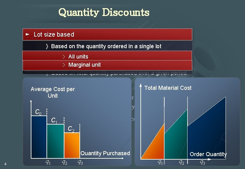
Quantity Discounts ► Lot size based 》Based on the quantity ordered in a single lot > All units ► Volume based > Marginal unit 》Based on total quantity purchased over a given period Total Material Cost Average Cost per Unitshould buyer react? How does this decision affect the supply chain E How in terms of lot sizes, cycle inventory, and flow time? C 0 What C 1 are appropriate discounting schemes that suppliers should offer? C 2 Quantity Purchased 4 q 1 q 2 q 3 Order Quantity q 1 q 2 q 3

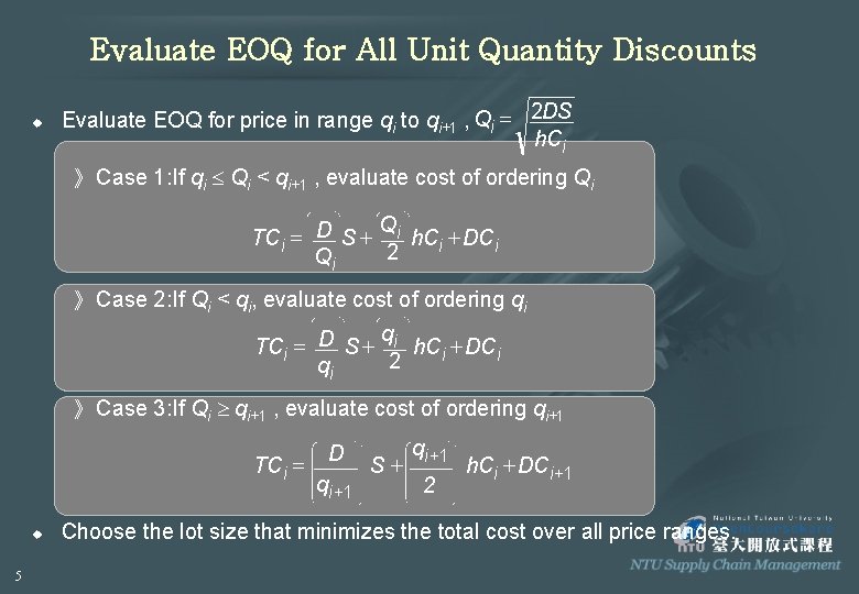
Evaluate EOQ for All Unit Quantity Discounts u Evaluate EOQ for price in range qi to qi+1 , Qi = 2 DS h. Ci 》 Case 1: If qi Qi < qi+1 , evaluate cost of ordering Qi Q TCi = D S + i h. Ci + DCi 2 Qi 》 Case 2: If Qi < qi, evaluate cost of ordering qi q TCi = D S + i h. Ci + DCi 2 qi 》 Case 3: If Qi qi+1 , evaluate cost of ordering qi+1 D TCi = S+ h. Ci + DCi+1 qi+1 2 u 5 Choose the lot size that minimizes the total cost over all price ranges.

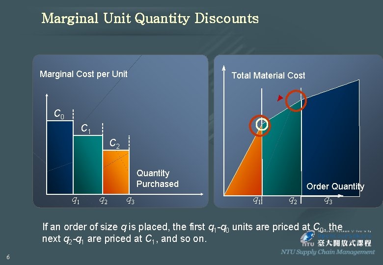
Marginal Unit Quantity Discounts Marginal Cost per Unit Total Material Cost C 0 C 1 C 2 Quantity Purchased q 1 q 2 q 3 Order Quantity q 1 q 2 q 3 If an order of size q is placed, the first q 1 -q 0 units are priced at C 0, the next q 2 -q 1 are priced at C 1, and so on. 6

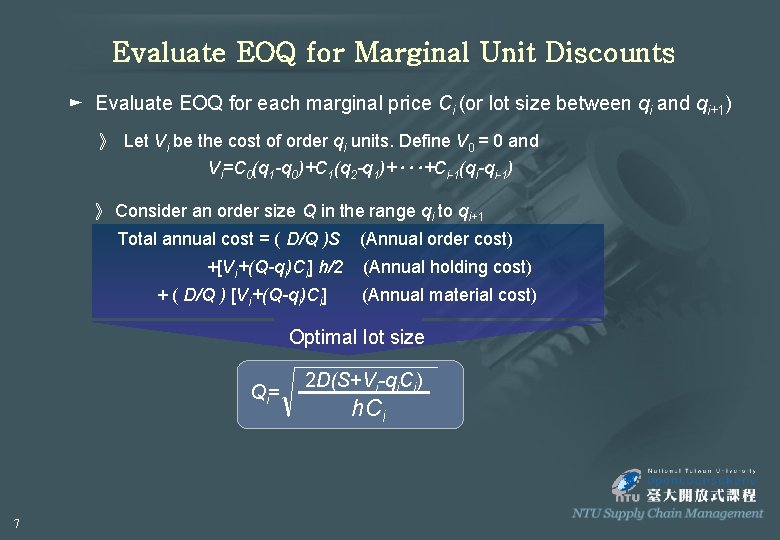
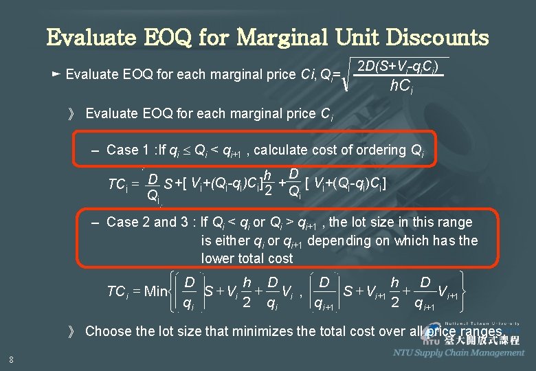
Evaluate EOQ for Marginal Unit Discounts ► Evaluate EOQ for each marginal price Ci (or lot size between qi and qi+1) 》 Let Vi be the cost of order qi units. Define V 0 = 0 and Vi=C 0(q 1 -q 0)+C 1(q 2 -q 1)+‧‧‧+Ci-1(qi-qi-1) 》 Consider an order size Q in the range qi to qi+1 Total annual cost = ( D/Q )S +[Vi+(Q-qi)Ci] h/2 + ( D/Q ) [Vi+(Q-qi)Ci] (Annual order cost) (Annual holding cost) (Annual material cost) Optimal lot size Qi= 7 2 D(S+Vi-qi. Ci) h. Ci

Evaluate EOQ for Marginal Unit Discounts ► Evaluate EOQ for each marginal price Ci, Qi= 2 D(S+Vi-qi. Ci) h. Ci 》 Evaluate EOQ for each marginal price Ci – Case 1 : If qi Qi < qi+1 , calculate cost of ordering Qi h D TCi = D S +[ Vi+(Qi-qi)Ci] 2 + Q [ Vi+(Qi-qi)Ci] i Qi – Case 2 and 3 : If Qi < qi or Qi > qi+1 , the lot size in this range is either qi or qi+1 depending on which has the lower total cost ì D ü h D D h D TCi = Miní S + Vi , S + Vi +1 ý 2 qi qi +1 2 q i +1 î qi þ 》 Choose the lot size that minimizes the total cost over all price ranges. 8

The Comparison between All Unit and Marginal Unit Quantity Discounts u u 9 The order quantity of all unit quantity discounts is less than the order quantity of marginal unit quantity discounts. The marginal unit quantity discounts will further enlarge the cycle inventory and average flow time.

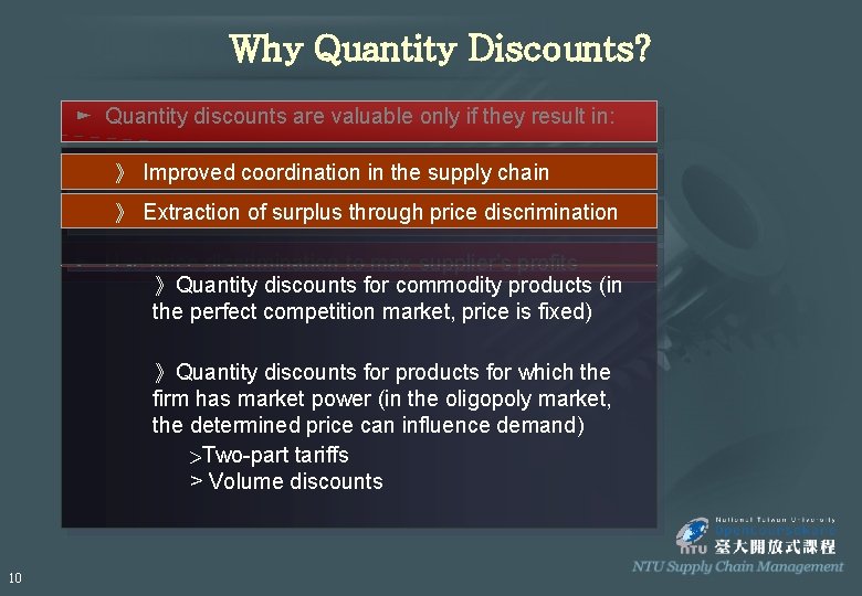
Why Quantity Discounts? ► Quantity discounts are valuable only if they result in: ► Coordination: max total profits of supply suppliers and retailers 》 Improved coordination in the chain 》 Extractioninofthe surplus through ► Coordination supply chain price discrimination ► Use price discrimination to max supplier’s profits 》Quantity discounts for commodity products (in the perfect competition market, price is fixed) 》Quantity discounts for products for which the firm has market power (in the oligopoly market, the determined price can influence demand) >Two-part tariffs > Volume discounts 10

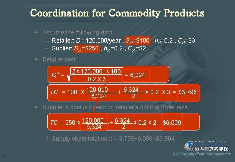
Coordination for Commodity Products ► Assume the following data. – Retailer: D =120, 000/year , SR=$100 , h. R=0. 2 , CR=$3 – Suplier: SS =$250 , h. S =0. 2 , CS =$2 ► Retailer cost Q* = 2 x 120, 000 x 100 = 6, 324 0. 2 x 3 TC = 100 x 120, 000 6, 324 + 6, 324 2 x 0. 2 x 3 = $3, 795 ► Supplier’s cost is based on retailer’s optimal order size. TC = 250 x 120, 000 6, 324 + 6, 324 x 0. 2 x 2 = $6, 009 2 》 Supply chain total cost = 3, 795+6, 009=$9, 804 11

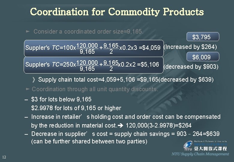
Coordination for Commodity Products ► Consider a coordinated order size=9, 165. $3, 795 Suppler's TC=100 x 120, 000 + 9, 165 x 0. 2 x 3 =$4, 059 (Increased by $264) 9, 165 2 $6, 009 Suppler's TC=250 x 120, 000 + 9, 165 x 0. 2 x 2 =$5, 106 (decreased by $903) 9, 165 2 》Supply chain total cost=4, 059+5, 106 =$9, 165(decreased by $639) ► Coordination through all unit quantity discounts. – $3 for lots below 9, 165 $2. 9978 for lots of 9, 165 or higher – Increase in retailer’s holding cost and order cost can be compensated by the reduction in material cost. 120, 000(3 -2. 9978)=$264 – Decrease in supplier’s cost = supply chain savings = 903– 264=$639 (can be further shared between two parties) 12

Coordination for Commodity Products u u 13 Since the price is determined by the market, supplier can use lotsize based quantity discounts to achieve coordination in supply chain and decrease supply chain cost. Lot size-based quantity discounts will increase cycle inventory. In theory, if supplier reduces its setup or order cost, the discount it offers will change and the cycle inventory is expected to decrease. In practice, the cycle inventory does not decrease in the supply chain because in most firms, marketing and sales department design quantity discounts independent of operations department who works on reducing the order cost.

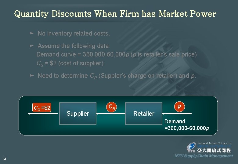
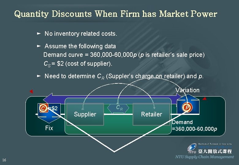
Quantity Discounts When Firm has Market Power ► No inventory related costs. ► Assume the following data Demand curve = 360, 000 -60, 000 p (p is retailer’s sale price) CS = $2 (cost of supplier). ► Need to determine CR (Suppler’s charge on retailer) and p. CS =$2 Supplier CR p Retailer Demand =360, 000 -60, 000 p 14

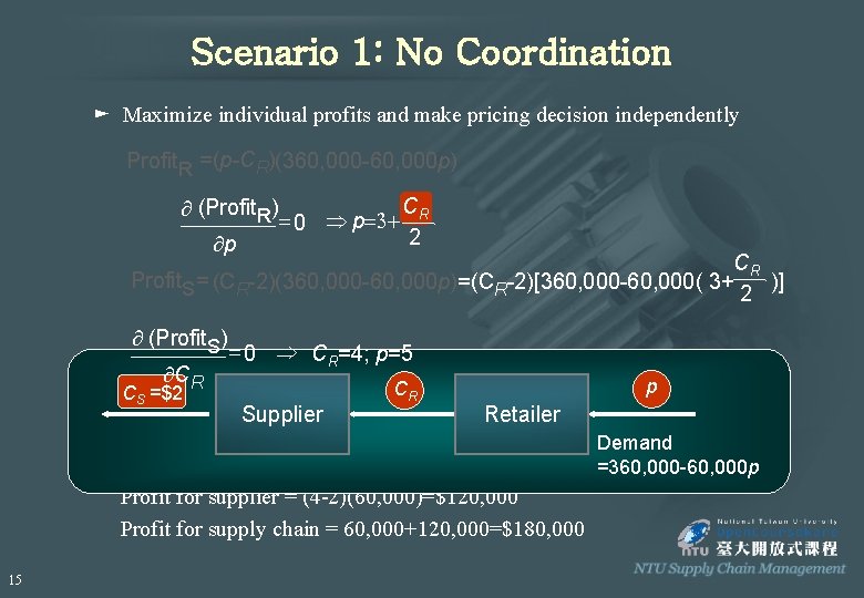
Scenario 1: No Coordination ► Maximize individual profits and make pricing decision independently Profit. R =(p-CR)(360, 000 -60, 000 p) C ¶ (Profit. R) = 0 Þ p=3+ R 2 ¶p CR Profit. S= (CR-2)(360, 000 -60, 000 p)=(CR-2)[360, 000 -60, 000( 3+ )] 2 ¶ (Profit. S) ¶CR CS =$2 = 0 Þ CR=4; p=5 CR p Supplier Retailer ► Demand = 360, 000 -60, 000(5)=60, 000 Demand Profit for retailer = (5 -4)(60, 000)=$60, 000 =360, 000 -60, 000 p Profit for supplier = (4 -2)(60, 000)=$120, 000 Profit for supply chain = 60, 000+120, 000=$180, 000 15

Quantity Discounts When Firm has Market Power ► No inventory related costs. ► Assume the following data Demand curve = 360, 000 -60, 000 p (p is retailer’s sale price) CS = $2 (cost of supplier). ► Need to determine CR (Suppler’s charge on retailer) and p. Variation CS =$2 Fix 16 Supplier CR p Retailer Demand =360, 000 -60, 000 p

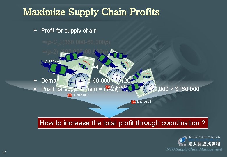
Maximize Supply Chain Profits ► Profit for supply chain =(p-Cs) (360, 000 -60, 000 p) =(p-2) (360, 000 -60, 000 p) ¶ (Profit) ¶p = 0 Þ p=4 ► Demand = 360, 000 -60, 000(4)=120, 000 Microsoft。 ► Profit for supple chain = (4 -2)(120, 000)=$240, 000 > $180, 000 Microsoft。 How to increase the total profit through coordination ? 17

Scenario 2: Coordination through Two-Part Tariff -I ► Supplier charges his entire profit as an up-front franchise fee. Supplier sells to the retailer at production cost (CS). ► Proof: Assume demand function = a-bp (a, b are constants) Then retailer’s profit = (p-c. R)(a-bp)-F (F: franchise fee) The supply chain’s profit = (p-c. S)(a-bp) Maximize both profits will obtain 18

Scenario 2: Coordination through Two-Part Tariff-II ► Supplier charges his entire profit as an up-front franchise fee. Supplier sells to the retailer at production cost (CS). ► Proof: Assume demand function = a-bp (a, b are constants) Then retailer’s profit = (p-c. R)(a-bp)-F (F: franchise fee) The supply chain’s profit = (p-c. S)(a-bp) Maximize both profits will obtain 19

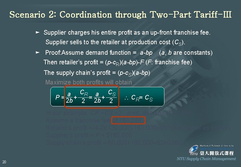
Scenario 2: Coordination through Two-Part Tariff-III ► Supplier charges his entire profit as an up-front franchise fee. Supplier sells to the retailer at production cost (CS). ► Proof: Assume demand function = a-bp (a, b are constants) Then retailer’s profit = (p-c. R)(a-bp)-F (F: franchise fee) The supply chain’s profit = (p-c. S)(a-bp) Maximize both profits will obtain a CR a CS P = 2 b + = + 2 2 b 2 C R= CS In our example, CR =CS =2 , p =4, demand=120, 000 Assume a franchise fee of 180, 000 Retailer’s profit =(4 -2)(120, 000)-180, 000=$60, 000 (same as before) Supplier’s profit = F = $180, 000 Supply chain’s profit = 60, 000+180, 000=$240, 000 20

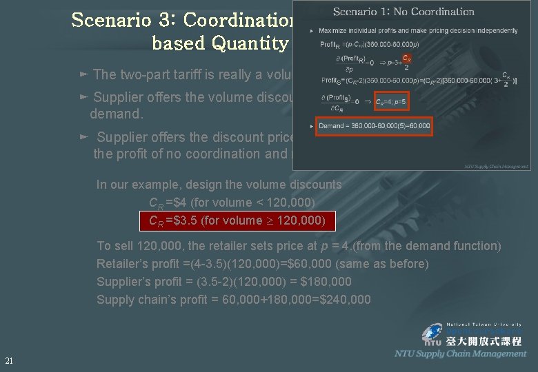
Scenario 3: Coordination through Volumebased Quantity Discounts ► The two-part tariff is really a volume-based quantity discounts. ► Supplier offers the volume discounts at the break point of optimal demand. ► Supplier offers the discount price so that the retailer will have a profit the profit of no coordination and no discount. In our example, design the volume discounts CR =$4 (for volume < 120, 000) CR =$3. 5 (for volume 120, 000) To sell 120, 000, the retailer sets price at p = 4. (from the demand function) Retailer’s profit =(4 -3. 5)(120, 000)=$60, 000 (same as before) Supplier’s profit = (3. 5 -2)(120, 000) = $180, 000 Supply chain’s profit = 60, 000+180, 000=$240, 000 21

Lessons From Discounting Schemes u u u Lot size-based discounts increase lot size and cycle inventory in the supply chain. Lot size-based discounts are justified to achieve coordination for commodity products. Volume-based discounts with some fixed cost passed on to retailer are more effective in general Volume-based discounts are better using rolling horizon to avoid the “hockey stick phenomenon”. u 22

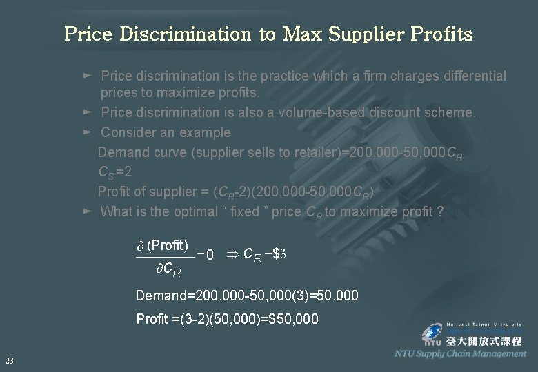
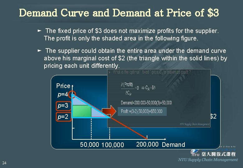
Price Discrimination to Max Supplier Profits ► Price discrimination is the practice which a firm charges differential prices to maximize profits. ► Price discrimination is also a volume-based discount scheme. ► Consider an example Demand curve (supplier sells to retailer)=200, 000 -50, 000 CR CS =2 Profit of supplier = (CR-2)(200, 000 -50, 000 CR) ► What is the optimal “ fixed ” price CR to maximize profit ? ¶ (Profit) ¶CR = 0 Þ CR =$3 Demand=200, 000 -50, 000(3)=50, 000 Profit =(3 -2)(50, 000)=$50, 000 23

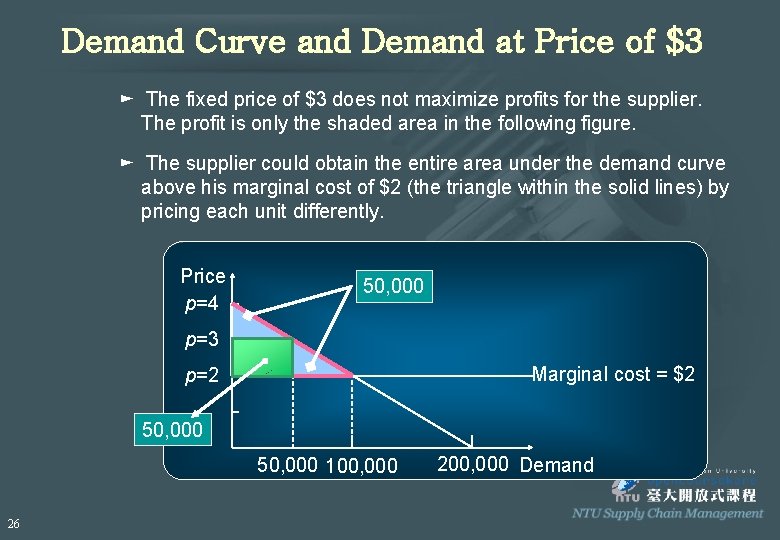
Demand Curve and Demand at Price of $3 ► The fixed price of $3 does not maximize profits for the supplier. The profit is only the shaded area in the following figure. ► The supplier could obtain the entire area under the demand curve above his marginal cost of $2 (the triangle within the solid lines) by pricing each unit differently. Price p=4 p=3 Marginal cost = $2 p=2 50, 000 100, 000 24 200, 000 Demand

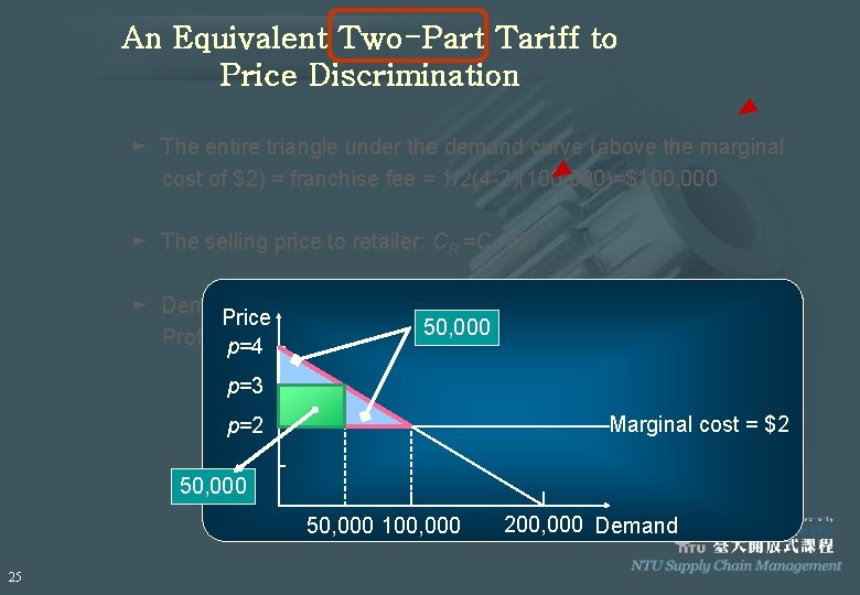
An Equivalent Two-Part Tariff to Price Discrimination ► The entire triangle under the demand curve (above the marginal cost of $2) = franchise fee = 1/2(4 -2)(100, 000)=$100, 000 ► The selling price to retailer: CR =CS =2. ► Demand = 200, 000 -50, 000(2)=100, 000 Price 50, 000 Profit of supplier = F = $100, 000 p=4 p=3 Marginal cost = $2 p=2 50, 000 100, 000 25 200, 000 Demand

Demand Curve and Demand at Price of $3 ► The fixed price of $3 does not maximize profits for the supplier. The profit is only the shaded area in the following figure. ► The supplier could obtain the entire area under the demand curve above his marginal cost of $2 (the triangle within the solid lines) by pricing each unit differently. Price p=4 50, 000 p=3 Marginal cost = $2 p=2 50, 000 100, 000 26 200, 000 Demand

Holding Cycle Inventory for Economies of Scale ► Fixed costs associated with lots ► Quantity discounts ► Trade Promotions 27

Trade Promotion ► Goals: – Induce retailers to spur sales – Shift inventory from manufacture to retailer and the customer – Defend a brand against competition ► Retailer options: – Pass through some or all of the promotion to customers to spur sales – Pass through very little of the promotion to customers but purchase in greater quantity to exploit temporary reduction in price (forward buying) 28

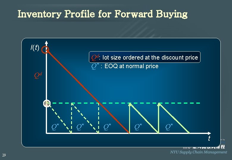
Inventory Profile for Forward Buying I(t) Qd: lot size ordered at the discount price Q* : EOQ at normal price Qd Q* Q* Q* t 29

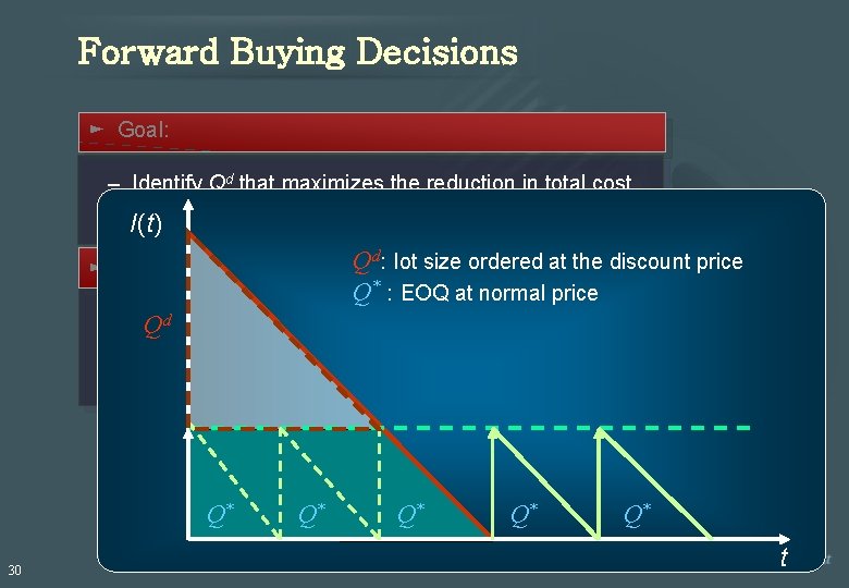
Forward Buying Decisions ► Goal: – Identify Qd that maximizes the reduction in total cost (material cost + order cost + holding cost) I(t) Qd: lot size ordered at the discount price Q* : EOQ at normal price ► Assumptions: – – – Discount will only be offered once. Qd Order quantity Qd is a multiple of Q*. The retailer takes no action to influence the demand. Q* 30 Q* Q* t

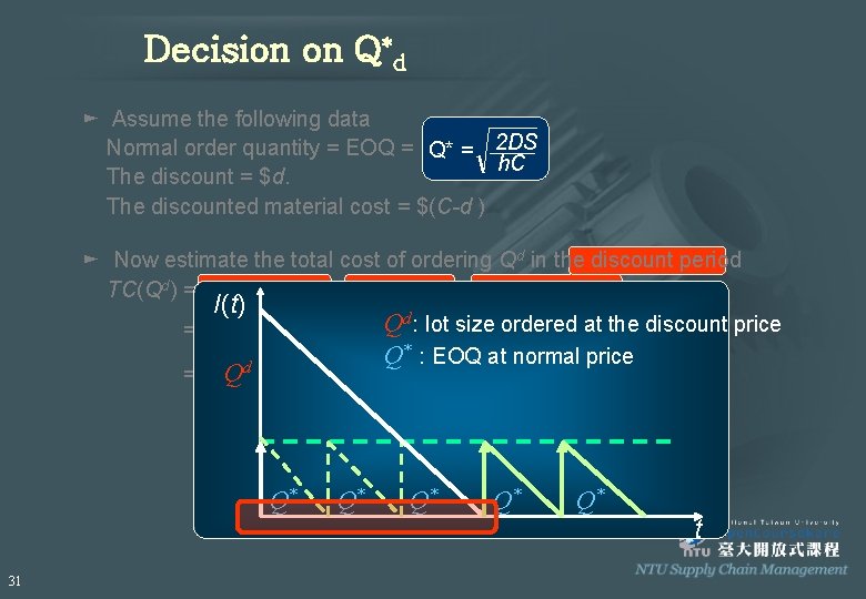
Decision on Q*d ► Assume the following data Normal order quantity = EOQ = Q* = 2 DS h. C The discount = $d. The discounted material cost = $(C-d ) ► Now estimate the total cost of ordering Qd in the discount period TC(Qd) = material cost + order cost + inventory cost I(t) d: lot sized ordered at the discount price =(C-d)Qd + S + Qd/2 Q (C-d)h [ Q /D ] * : EOQ at normal price Q Qd d + S + (Qd/D)2 (C-d)h / 2 D =(C-d)Q Note: Discount period =Qd/D Q* 31 Q* Q* t

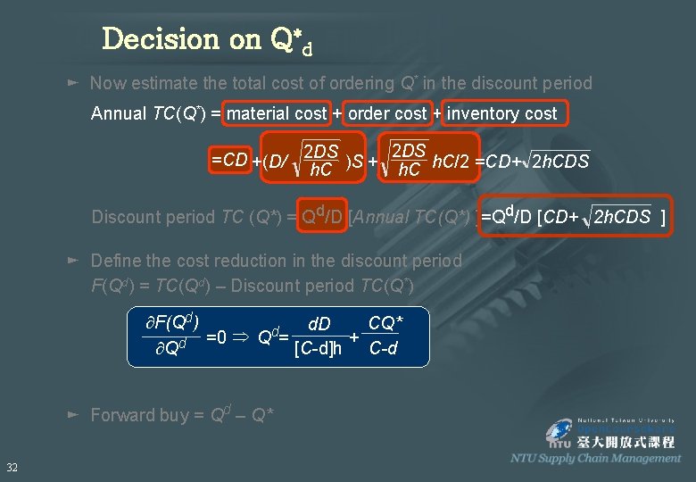
Decision on Q*d ► Now estimate the total cost of ordering Q* in the discount period Annual TC(Q*) = material cost + order cost + inventory cost =CD +(D/ 2 DS )S + 2 DS h. C/2 =CD+ 2 h. CDS h. C Discount period TC (Q*) = Qd/D [Annual TC(Q*) ]=Qd/D [CD+ 2 h. CDS ] ► Define the cost reduction in the discount period F(Qd) = TC(Qd) – Discount period TC(Q*) ¶F(Qd) CQ* d. D d Þ =0 Q = + ¶Qd [C-d]h C-d ► Forward buy = Qd – Q* 32

Decision on Q*d ► Now estimate the total cost of ordering Q* in the discount period Annual TC(Q*) = material cost + order cost + inventory cost =CD +(D/ 2 DS )S + 2 DS h. C/2 =CD+ 2 h. CDS h. C Discount period TC (Q*) = Qd/D [Annual TC(Q*) ]=Qd/D [CD+ 2 h. CDS ] ► Define the cost reduction in the discount period F(Qd) = TC(Qd) – Discount period TC(Q*) ¶F(Qd) CQ* d. D d Þ =0 Q = + ¶Qd [C-d]h C-d ► Forward buy = Qd – Q* 33

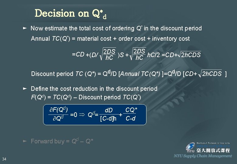
Decision on Q*d ► Now estimate the total cost of ordering Q* in the discount period Annual TC(Q*) = material cost + order cost + inventory cost =CD +(D/ 2 DS )S + 2 DS h. C/2 =CD+ 2 h. CDS h. C Discount period TC (Q*) = Qd/D [Annual TC(Q*) ]=Qd/D [CD+ 2 h. CDS ] ► Define the cost reduction in the discount period F(Qd) = TC(Qd) – Discount period TC(Q*) ¶F(Qd) CQ* d. D d Þ =0 Q = + ¶Qd [C-d]h C-d ► Forward buy = Qd – Q* 34

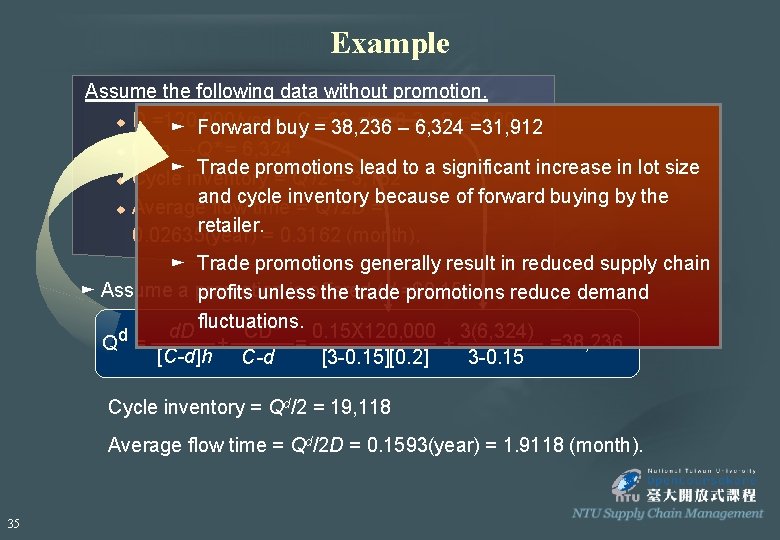
Example Assume the following data without promotion. u D =120, 000/year , C =$3 , h =0. 2 , S =$100 ► Forward buy = 38, 236 – 6, 324 =31, 912 u then →Q* = 6, 324 ► Trade promotions lead to a significant increase in lot size * u Cycle inventory = Q /2 = 3, 162 and cycle inventory because of forward buying by the * u Average flow time = Q /2 D = retailer. 0. 02635(year) = 0. 3162 (month). ► Trade promotions generally result in reduced supply chain ► Assume a promotion is offered (d =$0. 15) profits unless the trade promotions reduce demand fluctuations. d. D CD* 0. 15 X 120, 000 3(6, 324) =38, 236 Qd = + [C-d]h C-d [3 -0. 15][0. 2] 3 -0. 15 Cycle inventory = Qd/2 = 19, 118 Average flow time = Qd/2 D = 0. 1593(year) = 1. 9118 (month). 35

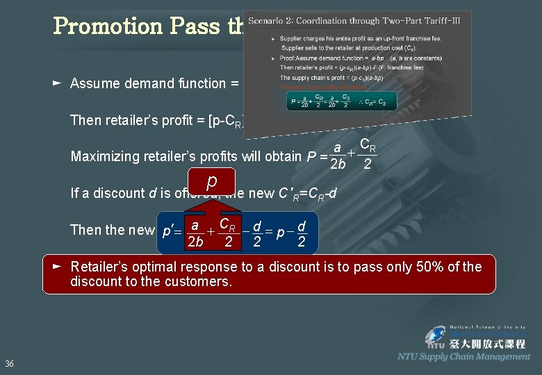
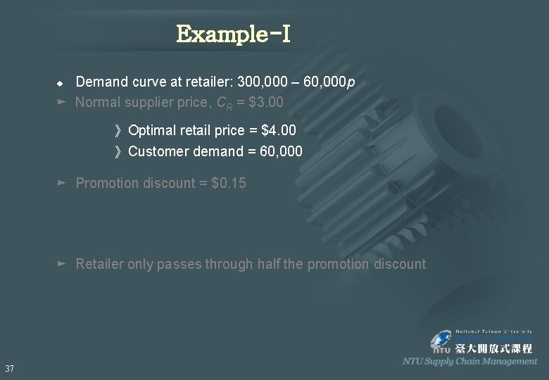
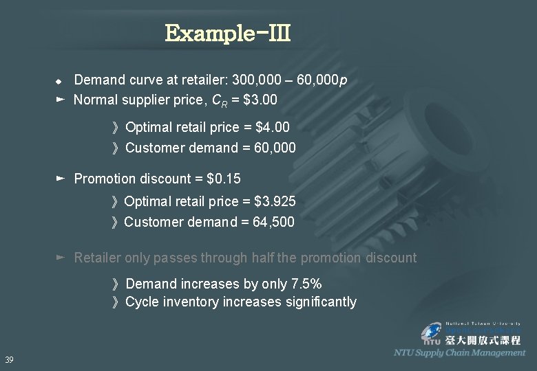
Promotion Pass through to Customers ► Assume demand function = a-bp (a, b are constants) Then retailer’s profit = [p-CR][a-bp] a + CR Maximizing retailer’s profits will obtain P = 2 b 2 p If a discount d is offered, the new C ¢R=CR-d Then the new p ¢= a + CR - d = p - d 2 2 2 b 2 ► Retailer’s optimal response to a discount is to pass only 50% of the discount to the customers. 36

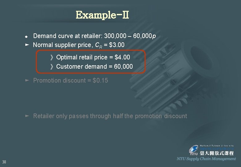
Example-I Demand curve at retailer: 300, 000 – 60, 000 p ► Normal supplier price, CR = $3. 00 u 》Optimal retail price = $4. 00 》Customer demand = 60, 000 ► Promotion discount = $0. 15 ► Retailer only passes through half the promotion discount 37

Example-II Demand curve at retailer: 300, 000 – 60, 000 p ► Normal supplier price, CR = $3. 00 u 》Optimal retail price = $4. 00 》Customer demand = 60, 000 ► Promotion discount = $0. 15 ► Retailer only passes through half the promotion discount 38

Example-III Demand curve at retailer: 300, 000 – 60, 000 p ► Normal supplier price, CR = $3. 00 u 》Optimal retail price = $4. 00 》Customer demand = 60, 000 ► Promotion discount = $0. 15 》Optimal retail price = $3. 925 》Customer demand = 64, 500 ► Retailer only passes through half the promotion discount 》Demand increases by only 7. 5% 》Cycle inventory increases significantly 39

Trade Promotions Goal is to discourage forward buying in the supply chain Counter measures – EDLP – Scan based promotions – Customer coupons Wikipedia Microsoft。 40

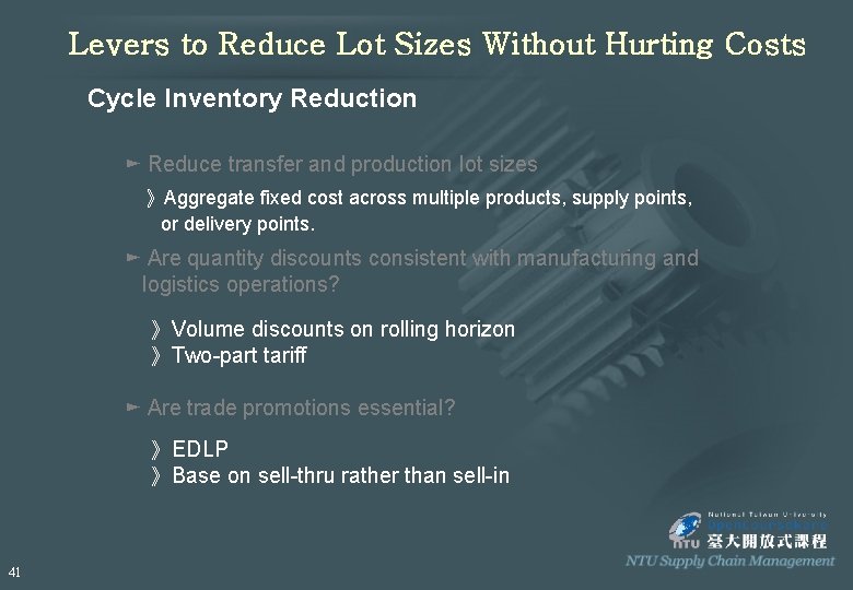
Levers to Reduce Lot Sizes Without Hurting Costs Cycle Inventory Reduction ► Reduce transfer and production lot sizes 》Aggregate fixed cost across multiple products, supply points, or delivery points. ► Are quantity discounts consistent with manufacturing and logistics operations? 》Volume discounts on rolling horizon 》Two-part tariff ► Are trade promotions essential? 》EDLP 》Base on sell-thru rather than sell-in 41