Chapter 4 Transient Heat Conduction Yoav Peles Department

Chapter 4: Transient Heat Conduction Yoav Peles Department of Mechanical, Aerospace and Nuclear Engineering Rensselaer Polytechnic Institute Copyright © The Mc. Graw-Hill Companies, Inc. Permission required for reproduction or display.

Objectives When you finish studying this chapter, you should be able to: • Assess when the spatial variation of temperature is negligible, and temperature varies nearly uniformly with time, making the simplified lumped system analysis applicable, • Obtain analytical solutions for transient one-dimensional conduction problems in rectangular, cylindrical, and spherical geometries using the method of separation of variables, and understand why a one-term solution is usually a reasonable approximation, • Solve the transient conduction problem in large mediums using the similarity variable, and predict the variation of temperature with time and distance from the exposed surface, and • Construct solutions for multi-dimensional transient conduction problems using the product solution approach.

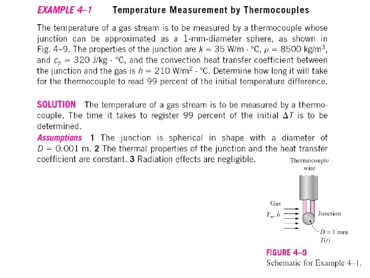
Lumped System Analysis • In heat transfer analysis, some bodies are essentially isothermal and can be treated as a “lump” system. • An energy balance of an isothermal solid for the time interval dt can be expressed as A s Heat Transfer into the body during dt = h SOLID BODY T∞ m=mass V=volume r=density Ti=initial temperature The increase in the energy of the body during dt T=T(t) h. As(T∞-T)dt=mcpd. T (4– 1)

• Noting that m=r. V and d. T=d(T-T∞) since T∞ constant, Eq. 4– 1 can be rearranged as (4– 2) • Integrating from time zero (at which T=Ti) to t gives (4– 3) • Taking the exponential of both sides and rearranging (4– 4) • b is a positive quantity whose dimension is (time)-1, and is called the time constant.

There are several observations that can be made from this figure and the relation above: 1. Equation 4– 4 enables us to determine the temperature T(t) of a body at time t, or alternatively, the time t required for the temperature to reach a specified value T(t). 2. The temperature of a body approaches the ambient temperature T exponentially. 3. The temperature of the body changes rapidly at the beginning, but rather slowly later on. 4. A large value of b indicates that the body approaches the ambient temperature in a short time.

Rate of Convection Heat Transfer • The rate of convection heat transfer between the body and the ambient can be determined from Newton’s law of cooling (4– 6) • The total heat transfer between the body and the ambient over the time interval 0 to t is simply the change in the energy content of the body: (4– 7) • The maximum heat transfer between the body and its surroundings (when the body reaches T∞) (4– 8)

Criteria for Lumped System Analysis • Assuming lumped system is not always appropriate, the first step in establishing a criterion for the applicability is to define a characteristic length • and a Biot number (Bi) as • It can also be expressed as (4– 9) Conduction resistance within the body Convection resistance at the surface of the body T∞ Rconv h Ts Rcond Tin

• Lumped system analysis assumes a uniform temperature distribution throughout the body, which is true only when thermal resistance of the body to heat conduction is zero. • The smaller the Bi number, the more accurate the lumped system analysis. • It is generally accepted that lumped system analysis is applicable if

Transient Heat Conduction in Large Plane Walls, Long Cylinders, and Spheres with Spatial Effects • In many transient heat transfer problems the Biot number is larger than 0. 1, and lumped system can not be assumed. • In these cases the temperature within the body changes appreciably from point to point as well as with time. • It is constructive to first consider the variation of temperature with time and position in one-dimensional problems of rudimentary configurations such as a large plane wall, a long cylinder, and a sphere.

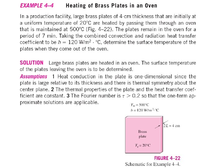
A large Plane Wall • A plane wall of thickness 2 L. • Initially at a uniform temperature of Ti. • At time t=0, the wall is immersed in a fluid at temperature T∞. • Constant heat transfer coefficient h. • The height and the width of the wall are large relative to its thickness one-dimensional approximation is valid. • Constant thermophysical properties. • No heat generation. • There is thermal symmetry about the midplane passing through x=0.

The Heat Conduction Equation • One-dimensional transient heat conduction equation problem (0≤ x ≤ L): Differential equation: (4– 10 a) Boundary conditions: (4– 10 b) Initial condition: (4– 10 c)

Nondimensional Equation • A dimensionless space variable X=x/L • A dimensionless temperature variable q(x, t)=[T(x, t)-T∞]/[Ti-T∞] • The dimensionless time and h/k ratio will be obtained through the analysis given below • Introducing the dimensionless variable into Eq. 4 -10 a • Substituting into Eqs. 4– 10 a and 4– 10 b and rearranging (4– 11)

• Therefore, the dimensionless time is t=at/L 2, which is called the Fourier number (Fo). • h. L/k is the Biot number (Bi). • The one-dimensional transient heat conduction problem in a plane wall can be expressed in nondimensional form as Differential equation: (4– 12 a) Boundary conditions: (4– 12 b) Initial condition: (4– 12 c)

Exact Solution • Several analytical and numerical techniques can be used to solve Eq. 4 -12. • We will use the method of separation of variables. • The dimensionless temperature function q(X, t) is expressed as a product of a function of X only and a function of t only as (4– 14) • Substituting Eq. 4– 14 into Eq. 4– 12 a and dividing by the product FG gives (4– 15)

• Since X and t can be varied independently, the equality in Eq. 4– 15 can hold for any value of X and t only if Eq. 4– 15 is equal to a constant. • It must be a negative constant that we will indicate by -l 2 since a positive constant will cause the function G(t) to increase indefinitely with time. • Setting Eq. 4– 15 equal to -l 2 gives (4– 16) • whose general solutions are (4– 17)

(4– 18) • where A=C 1 C 3 and B=C 2 C 3 are arbitrary constants. • Note that we need to determine only A and B to obtain the solution of the problem. • Applying the boundary conditions in Eq. 4– 12 b gives

• But tangent is a periodic function with a period of p, and the equation ltan(l)=Bi has the root l 1 between 0 and p, the root l 2 between p and 2 p, the root ln between (n-1)p and np, etc. • To recognize that the transcendental equation ltan(l)=Bi has an infinite number of roots, it is expressed as (4– 19) • Eq. 4– 19 is called the characteristic equation or eigenfunction, and its roots are called the characteristic values or eigenvalues. • It follows that there an infinite number of solutions of the form , and the solution of this linear heat conduction problem is a linear combination of them, (4– 20) • The constants An are determined from the initial condition, Eq. 4– 12 c, (4– 21)

• Multiply both sides of Eq. 4– 21 by cos(lm. X), and integrating from X=0 to X=1 • The right-hand side involves an infinite number of integrals of the form • It can be shown that all of these integrals vanish except when n=m, and the coefficient An becomes (4– 22)

• Substituting Eq. 4 -22 into Eq. 20 a gives • Where ln is obtained from Eq. 4 -19. • As demonstrated in Fig. 4– 14, the terms in the summation decline rapidly as n and thus ln increases. • Solutions in other geometries such as a long cylinder and a sphere can be determined using the same approach and are given in Table 4 -1. FIGURE 4 -14

Summary of the Solutions for One. Dimensional Transient Conduction

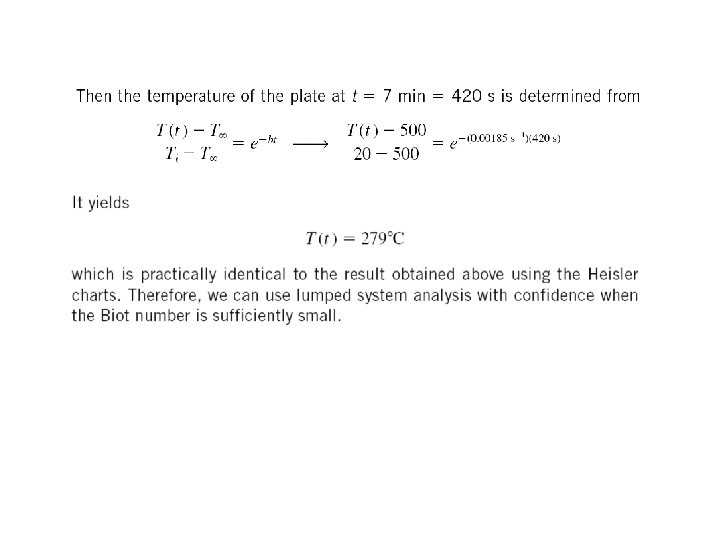
Approximate Analytical and Graphical Solutions • The series solutions of Eq. 4 -20 and in Table 4– 1 converge rapidly with increasing time, and for t >0. 2, keeping the first term and neglecting all the remaining terms in the series results in an error under 2 percent. • Thus for t >0. 2 the one-term approximation can be used Plane wall: (4– 23) Cylinder: (4– 24) Sphere: (4– 25)

• The constants A 1 and l 1 are functions of the Bi number only, and their values are listed in Table 4– 2 against the Bi number for all three geometries. • The function J 0 is the zeroth-order Bessel function of the first kind, whose value can be determined from Table 4– 3.

The solution at the center of a plane wall, cylinder, and sphere: Center of plane wall (x=0): (4– 26) Center of cylinder (r=0): (4– 27) Center of sphere (r=0): (4– 28)

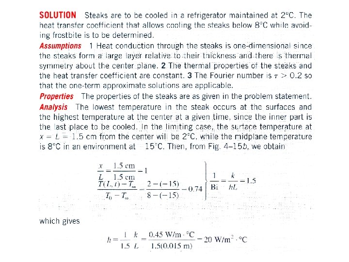
Heisler Charts • The solution of the transient temperature for a large plane wall, long cylinder, and sphere also presented in graphical form for t>0. 2, known as the transient temperature charts (also known as the Heisler Charts). • There are three charts associated with each geometry: – the temperature T 0 at the center of the geometry at a given time t. – the temperature at other locations at the same time in terms of T 0. – the total amount of heat transfer up to the time t.

Heisler Charts – Plane Wall Midplane temperature

Heisler Charts – Plane Wall Heat Transfer Temperature distribution

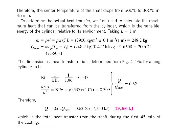
Heat Transfer • The maximum amount of heat that a body can gain (or lose if Ti=T∞) occurs when the temperature of the body is changes from the initial temperature Ti to the ambient temperature (4– 30) • The amount of heat transfer Q at a finite time t is can be expressed as (4– 31)

• Assuming constant properties, the ratio of Q/Qmax becomes (4– 32) • The following relations for the fraction of heat transfer in those geometries: Plane wall: (4– 33) Cylinder: (4– 34) Sphere: (4– 35)

Remember, the Heisler charts are not generally applicable The Heisler Charts can only be used when: • the body is initially at a uniform temperature, • the temperature of the medium surrounding the body is constant and uniform. • the convection heat transfer coefficient is constant and uniform, and there is no heat generation in the body.

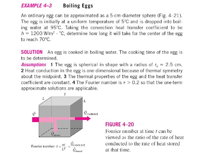
Fourier number The rate at which heat is conducted across L of a body of volume L 3 The rate at which heat is stored in a body of volume L 3 • The Fourier number is a measure of heat conducted through a body relative to heat stored. • A large value of the Fourier number indicates faster propagation of heat through a body.

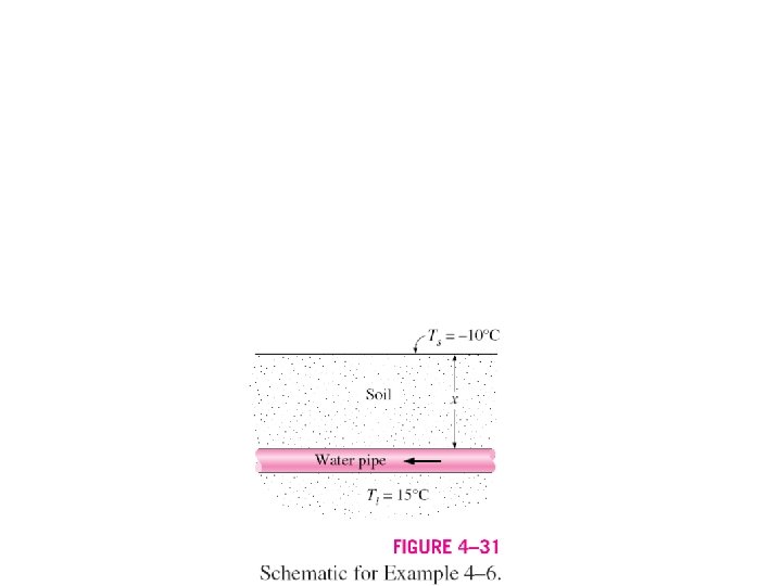
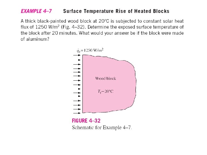
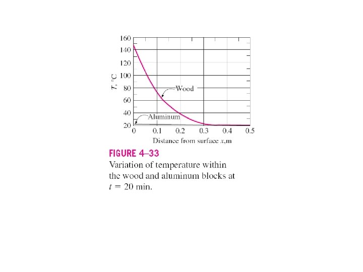
Transient Heat Conduction in Semi. Infinite Solids • A semi-infinite solid is an idealized body that has a single plane surface and extends to infinity in all directions. • Assumptions: – – constant thermophysical properties no internal heat generation uniform thermal conditions on its exposed surface initially a uniform temperature of Ti throughout. • Heat transfer in this case occurs only in the direction normal to the surface (the x direction) one-dimensional problem.

• Eq. 4– 10 a for one-dimensional transient conduction in Cartesian coordinates applies Differential equation: Boundary conditions: Initial condition: (4– 10 a) (4– 37 b) (4– 10 c) • The separation of variables technique does not work in this case since the medium is infinite. • The partial differential equation can be converted into an ordinary differential equation by combining the two independent variables x and t into a single variable h, called the similarity variable.

Similarity Solution • For transient conduction in a semi-infinite medium Similarity variable: • Assuming T=T(h) (to be verified) and using the chain rule, all derivatives in the heat conduction equation can be transformed into the new variable (4– 39 a)

(4– 39 a) • Noting that h=0 at x=0 and h→∞ as x→∞ (and also at t=0) and substituting into Eqs. 4– 37 b (BC) give, after simplification (4– 39 b) • Note that the second boundary condition and the initial condition result in the same boundary condition. • Both the transformed equation and the boundary conditions depend on h only and are independent of x and t. Therefore, transformation is successful, and h is indeed a similarity variable.

• To solve the 2 nd order ordinary differential equation in Eqs. 4– 39, we define a new variable w as w=d. T/dh. This reduces Eq. 4– 39 a into a first order differential equation than can be solved by separating variables, • where C 1=ln(C 0). • Back substituting w=d. T/dh and integrating again, (4– 40) • where u is a dummy integration variable. The boundary condition at h=0 gives C 2=Ts, and the one for h→∞ gives (4– 41)

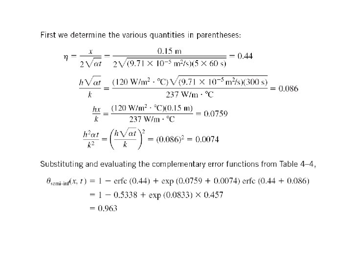
• Substituting the C 1 and C 2 expressions into Eq. 4– 40 and rearranging, (4– 42) • Where (4– 43) • are called the error function and the complementary error function, respectively, of argument h.

• Knowing the temperature distribution, the heat flux at the surface can be determined from the Fourier’s law to be (4– 44)

Other Boundary Conditions • The solutions in Eqs. 4– 42 and 4– 44 correspond to the case when the temperature of the exposed surface of the medium is suddenly raised (or lowered) to Ts at t=0 and is maintained at that value at all times. • Analytical solutions can be obtained for other boundary conditions on the surface and are given in the book – Specified Surface Temperature, Ts = constant. – Constant and specified surface heat flux. – Convection on the Surface, – Energy Pulse at Surface.

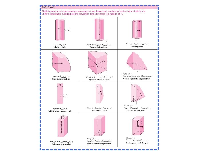
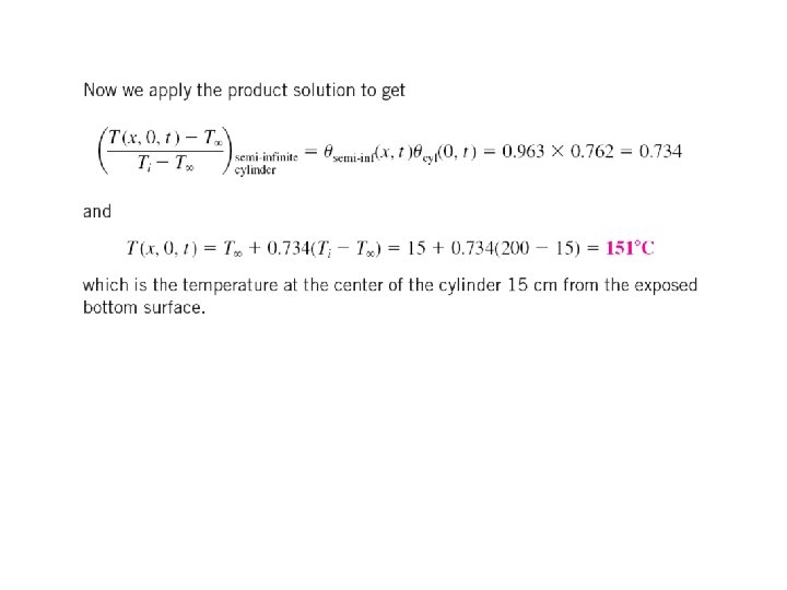
Transient Heat Conduction in Multidimensional Systems • Using a superposition approach called the product solution, the one-dimensional heat conduction solutions can also be used to construct solutions for some two-dimensional (and even three-dimensional) transient heat conduction problems. • Provided that all surfaces of the solid are subjected to convection to the same fluid at temperature, the same heat transfer coefficient h, and the body involves no heat generation.

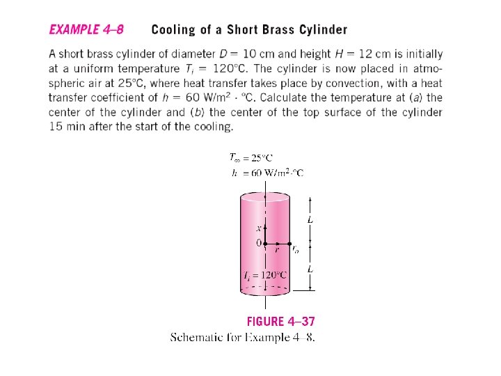
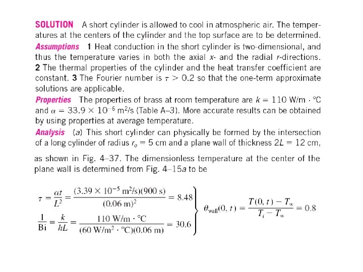
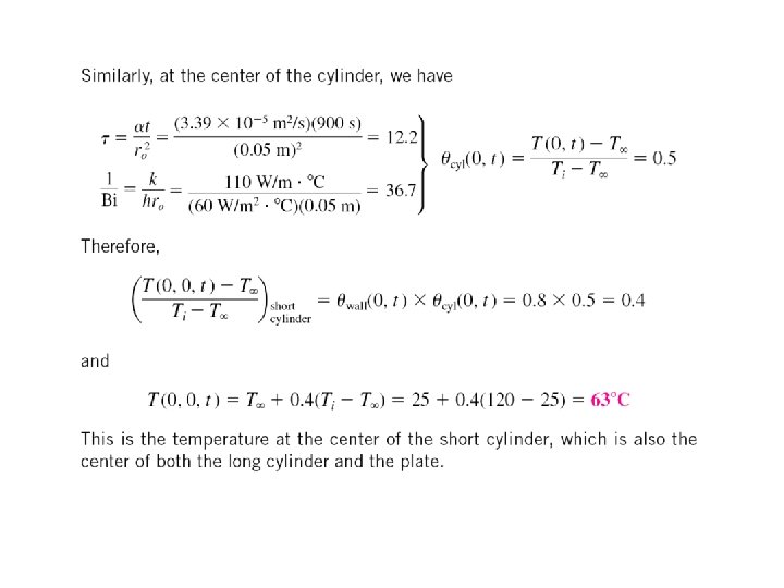
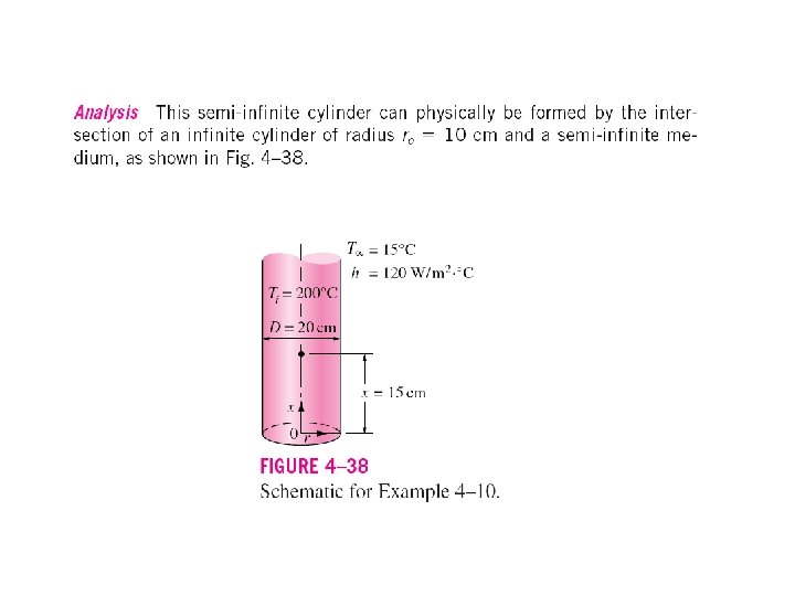
Example ─ short cylinder • • Height a and radius ro. Initially uniform temperature Ti. No heat generation At time t=0: – convection T∞ – heat transfer coefficient h • The solution: (4– 50)

• The solution can be generalized as follows: the solution for a multidimensional geometry is the product of the solutions of the one-dimensional geometries whose intersection is the multidimensional body. • For convenience, the one-dimensional solutions are denoted by (4– 51)

Total Transient Heat Transfer • The transient heat transfer for a two dimensional geometry formed by the intersection of two one-dimensional geometries 1 and 2 is: (4– 53) • Transient heat transfer for a three-dimensional (intersection of three one-dimensional bodies 1, 2, and 3) is: (4– 54)