CHAPTER 19 Series and Residues Contents v 19

CHAPTER 19 Series and Residues

Contents v 19. 1 Sequences and Series v 19. 2 Taylor Series v 19. 3 Laurent Series v 19. 4 Zeros and Poles v 19. 5 Residues and Residue Theorem v 19. 6 Evaluation of Real Integrals 2

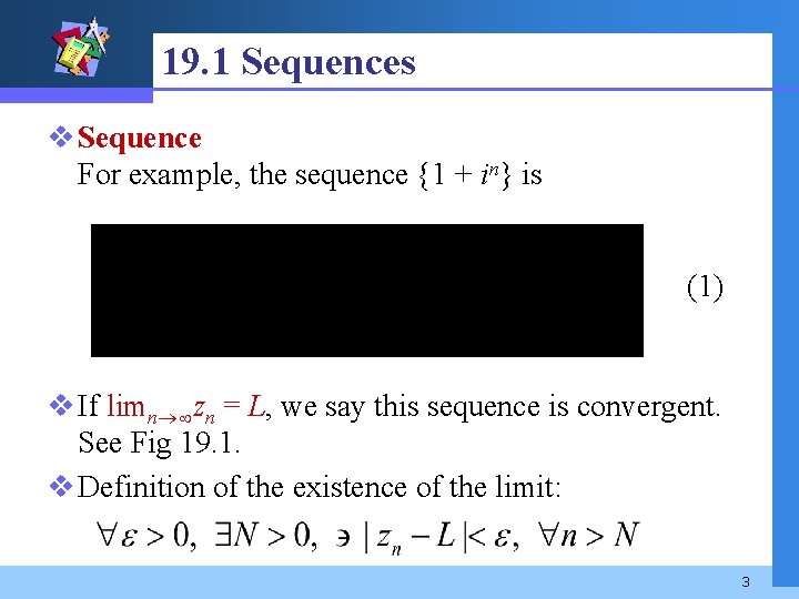
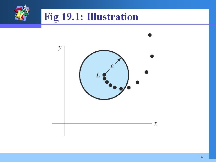
19. 1 Sequences v Sequence For example, the sequence {1 + in} is (1) v If limn zn = L, we say this sequence is convergent. See Fig 19. 1. v Definition of the existence of the limit: 3

Fig 19. 1: Illustration 4

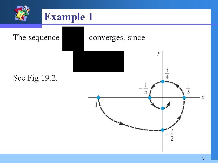
Example 1 The sequence converges, since See Fig 19. 2. 5

THEOREM 19. 1 Criterion for Convergence A sequence {zn} converge to a complex number L if and only if Re(zn) converges to Re(L) and Im(zn) converges to Im(L). 6

Example 2 The sequence converges to i. Note that Re(i) = 0 and Im(i) = 1. Then 7

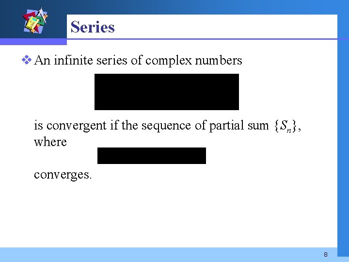
Series v An infinite series of complex numbers is convergent if the sequence of partial sum {Sn}, where converges. 8

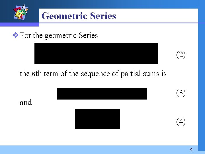
Geometric Series v For the geometric Series (2) the nth term of the sequence of partial sums is (3) and (4) 9

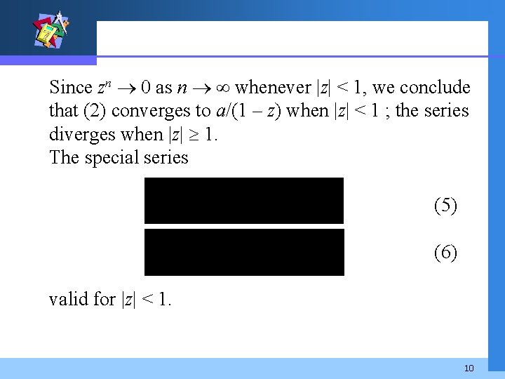
Since zn 0 as n whenever |z| < 1, we conclude that (2) converges to a/(1 – z) when |z| < 1 ; the series diverges when |z| 1. The special series (5) (6) valid for |z| < 1. 10

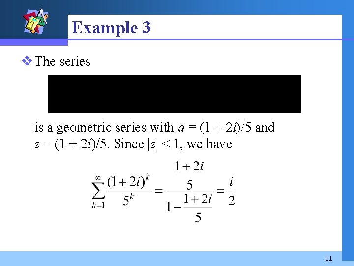
Example 3 v The series is a geometric series with a = (1 + 2 i)/5 and z = (1 + 2 i)/5. Since |z| < 1, we have 11

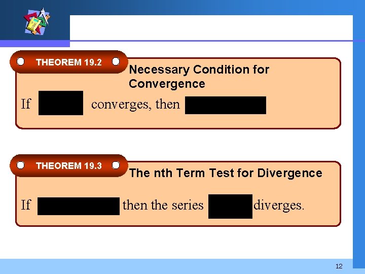
THEOREM 19. 2 If converges, then THEOREM 19. 3 If Necessary Condition for Convergence The nth Term Test for Divergence then the series diverges. 12

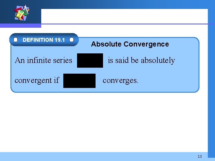
DEFINITION 19. 1 An infinite series convergent if Absolute Convergence is said be absolutely converges. 13

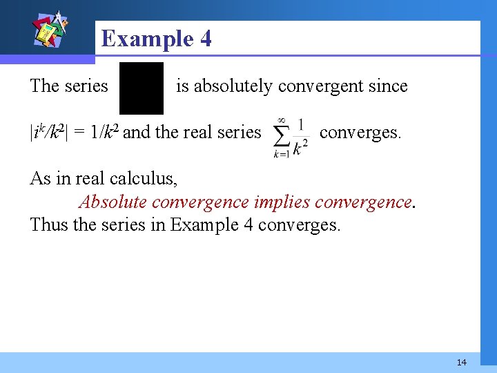
Example 4 The series is absolutely convergent since |ik/k 2| = 1/k 2 and the real series converges. As in real calculus, Absolute convergence implies convergence. Thus the series in Example 4 converges. 14

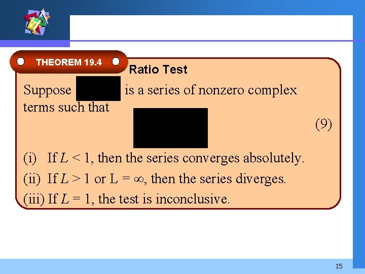
THEOREM 19. 4 Suppose terms such that Ratio Test is a series of nonzero complex (9) (i) If L < 1, then the series converges absolutely. (ii) If L > 1 or L = , then the series diverges. (iii) If L = 1, the test is inconclusive. 15

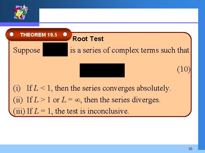
THEOREM 19. 5 Suppose Root Test is a series of complex terms such that (10) (i) If L < 1, then the series converges absolutely. (ii) If L > 1 or L = , then the series diverges. (iii) If L = 1, the test is inconclusive. 16

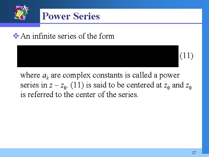
Power Series v An infinite series of the form (11) where ak are complex constants is called a power series in z – z 0. (11) is said to be centered at z 0 and z 0 is referred to the center of the series. 17

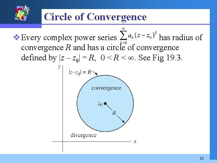
Circle of Convergence v Every complex power series has radius of convergence R and has a circle of convergence defined by |z – z 0| = R, 0 < R < . See Fig 19. 3. 18

v The radius R can be (i) zero (converges at only z = z 0). (ii) a finite number (converges at all interior points of the circle |z − z 0| = R). (iii) (converges for all z). A power series may converge at some, all, or none of the points on the circle of convergence. 19

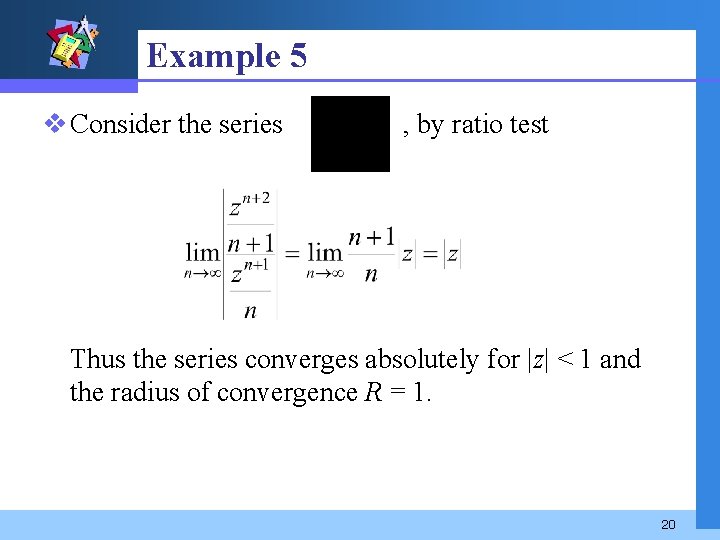
Example 5 v Consider the series , by ratio test Thus the series converges absolutely for |z| < 1 and the radius of convergence R = 1. 20

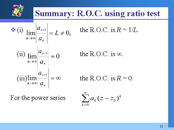
Summary: R. O. C. using ratio test v (i) the R. O. C. is R = 1/L. (ii) the R. O. C. is . (iii) the R. O. C. is R = 0. For the power series 21

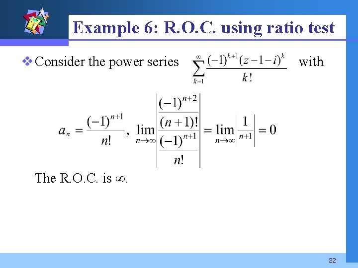
Example 6: R. O. C. using ratio test v Consider the power series with The R. O. C. is . 22

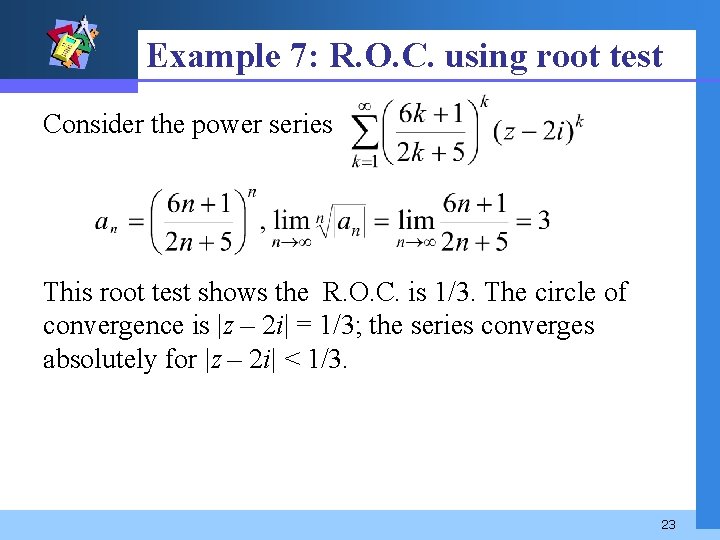
Example 7: R. O. C. using root test Consider the power series This root test shows the R. O. C. is 1/3. The circle of convergence is |z – 2 i| = 1/3; the series converges absolutely for |z – 2 i| < 1/3. 23

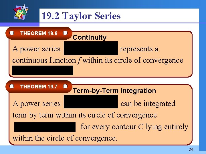
19. 2 Taylor Series THEOREM 19. 6 Continuity A power series represents a continuous function f within its circle of convergence THEOREM 19. 7 Term-by-Term Integration A power series can be integrated term by term within its circle of convergence for every contour C lying entirely within the circle of convergence. 24

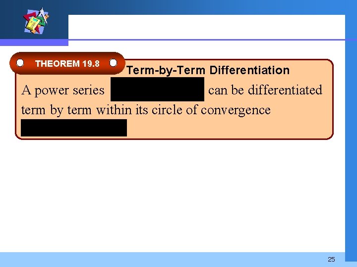
THEOREM 19. 8 Term-by-Term Differentiation A power series can be differentiated term by term within its circle of convergence 25

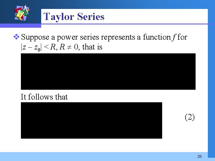
Taylor Series v Suppose a power series represents a function f for |z – z 0| < R, R 0, that is (1) It follows that (2) 26

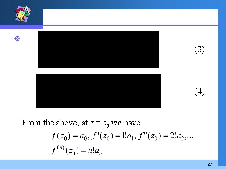
v (3) (4) From the above, at z = z 0 we have 27

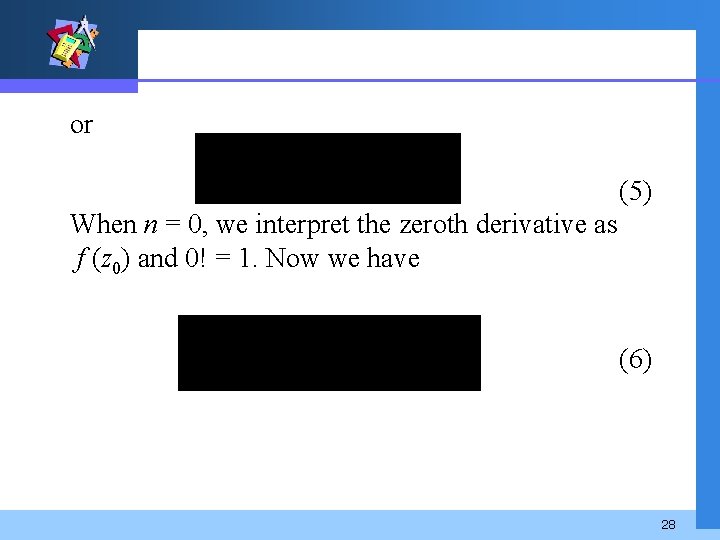
or (5) When n = 0, we interpret the zeroth derivative as f (z 0) and 0! = 1. Now we have (6) 28

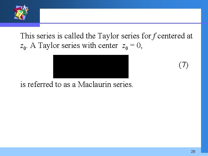
This series is called the Taylor series for f centered at z 0. A Taylor series with center z 0 = 0, (7) is referred to as a Maclaurin series. 29

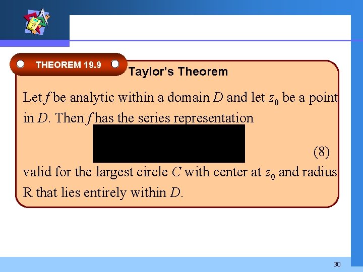
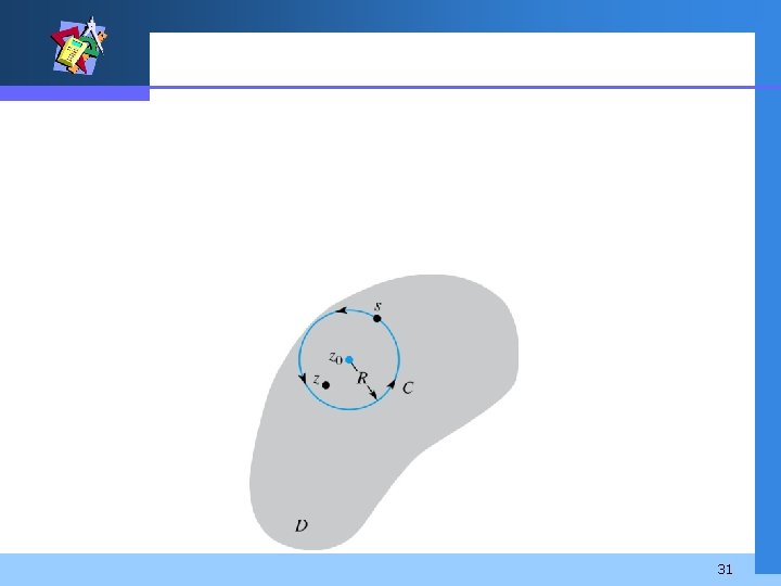
THEOREM 19. 9 Taylor’s Theorem Let f be analytic within a domain D and let z 0 be a point in D. Then f has the series representation (8) valid for the largest circle C with center at z 0 and radius R that lies entirely within D. 30

31

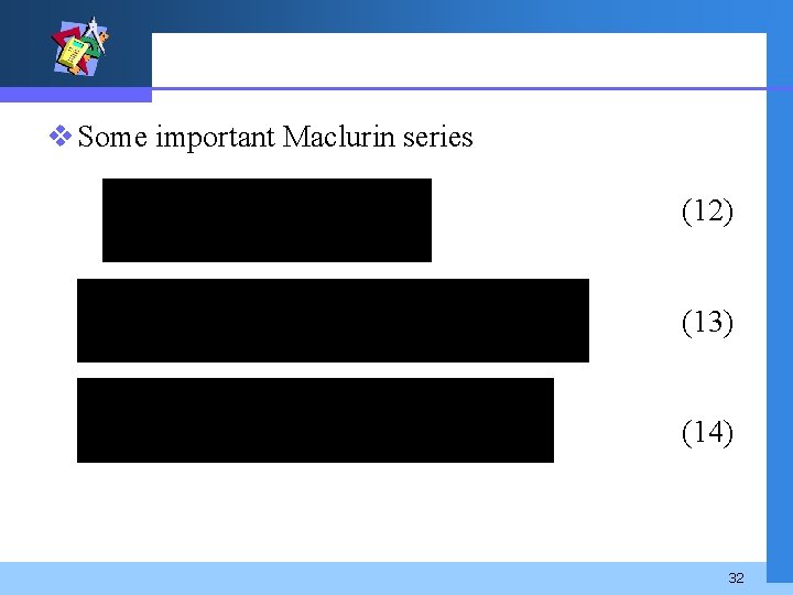
v Some important Maclurin series (12) (13) (14) 32

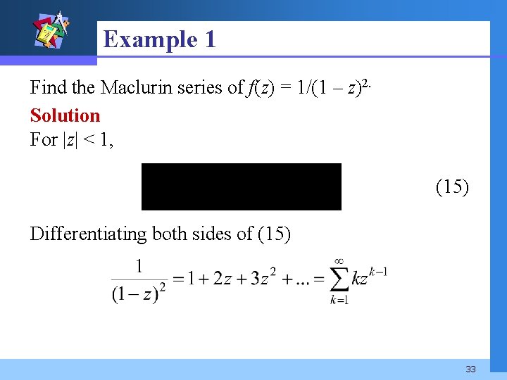
Example 1 Find the Maclurin series of f(z) = 1/(1 – z)2. Solution For |z| < 1, (15) Differentiating both sides of (15) 33

19. 3 Laurent Series v Isolated Singularities Suppose z = z 0 is a singularity of a complex function f. For example, 2 i and -2 i are sigularities of The point z 0 is said to be an isolated singularity, if there exists some deleted neighborhood or punctured open disk 0 < |z – z 0| < R throughout which is analytic. 34

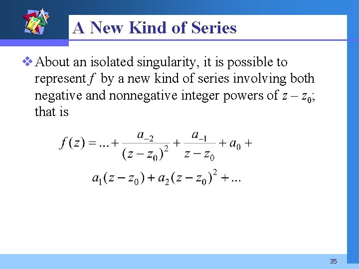
A New Kind of Series v About an isolated singularity, it is possible to represent f by a new kind of series involving both negative and nonnegative integer powers of z – z 0; that is 35

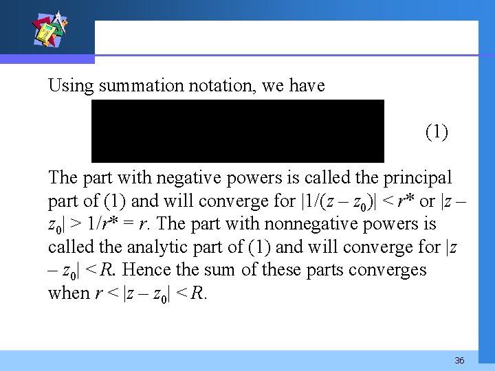
Using summation notation, we have (1) The part with negative powers is called the principal part of (1) and will converge for |1/(z – z 0)| < r* or |z – z 0| > 1/r* = r. The part with nonnegative powers is called the analytic part of (1) and will converge for |z – z 0| < R. Hence the sum of these parts converges when r < |z – z 0| < R. 36

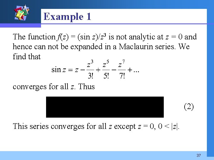
Example 1 The function f(z) = (sin z)/z 3 is not analytic at z = 0 and hence can not be expanded in a Maclaurin series. We find that converges for all z. Thus (2) This series converges for all z except z = 0, 0 < |z|. 37

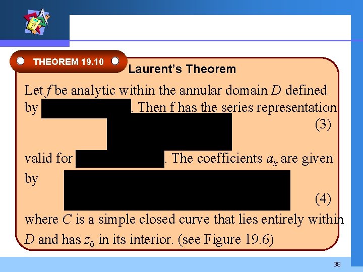
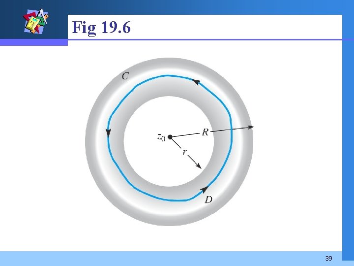
THEOREM 19. 10 Laurent’s Theorem Let f be analytic within the annular domain D defined by. Then f has the series representation (3) valid for by . The coefficients ak are given (4) where C is a simple closed curve that lies entirely within D and has z 0 in its interior. (see Figure 19. 6) 38

Fig 19. 6 39

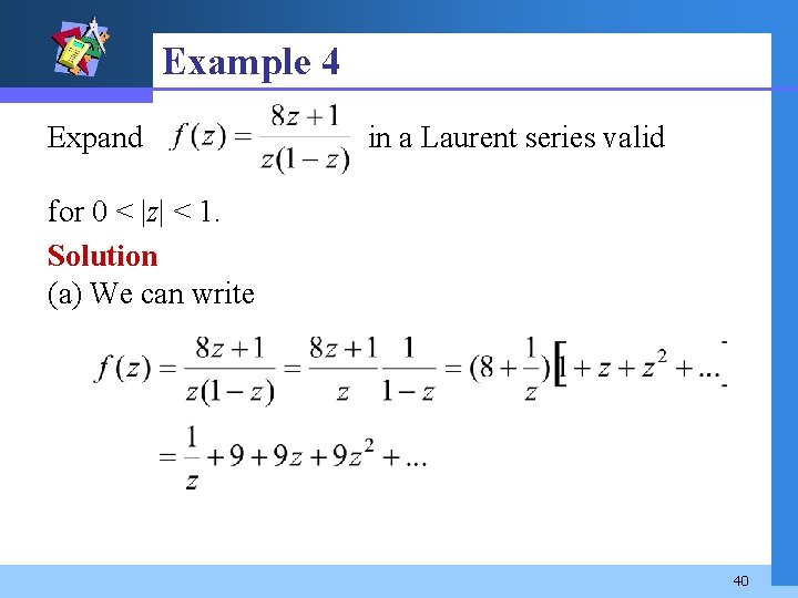
Example 4 Expand in a Laurent series valid for 0 < |z| < 1. Solution (a) We can write 40

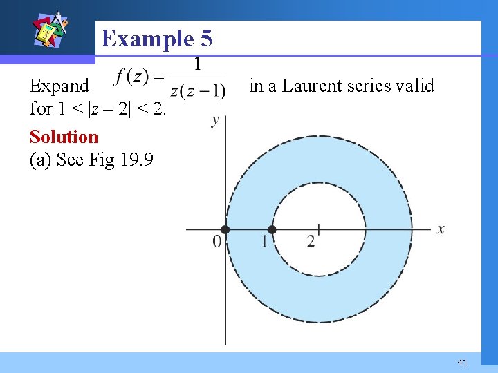
Example 5 Expand for 1 < |z – 2| < 2. Solution (a) See Fig 19. 9 in a Laurent series valid 41

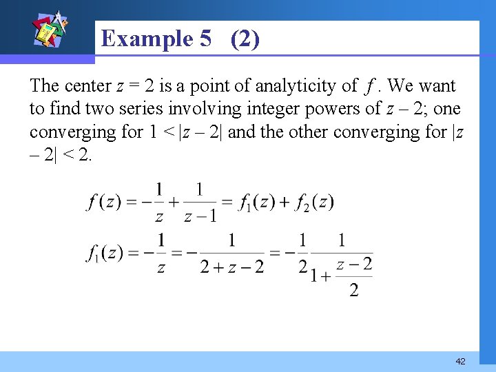
Example 5 (2) The center z = 2 is a point of analyticity of f. We want to find two series involving integer powers of z – 2; one converging for 1 < |z – 2| and the other converging for |z – 2| < 2. 42

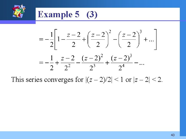
Example 5 (3) This series converges for |(z – 2)/2| < 1 or |z – 2| < 2. 43

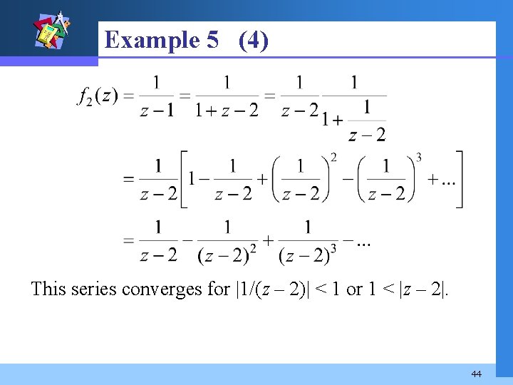
Example 5 (4) This series converges for |1/(z – 2)| < 1 or 1 < |z – 2|. 44

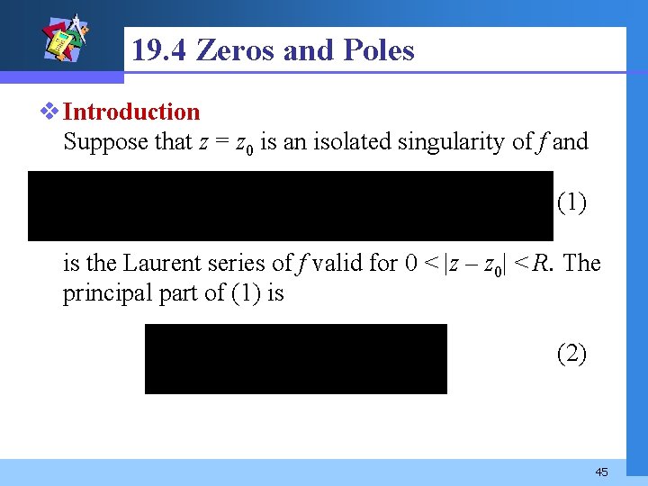
19. 4 Zeros and Poles v Introduction Suppose that z = z 0 is an isolated singularity of f and (1) is the Laurent series of f valid for 0 < |z – z 0| < R. The principal part of (1) is (2) 45

Classification (i) If the principal part is zero, z = z 0 is called a removable singularity. (ii) If the principal part contains a finite number of terms, then z = z 0 is called a pole. If the last nonzero coefficient is a-n, n 1, then we say it is a pole of order n. A pole of order 1 is commonly called a simple pole. (iii) If the principal part contains infinitely many nonzero terms, z = z 0 is called an essential singularity. 46

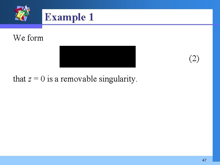
Example 1 We form (2) that z = 0 is a removable singularity. 47

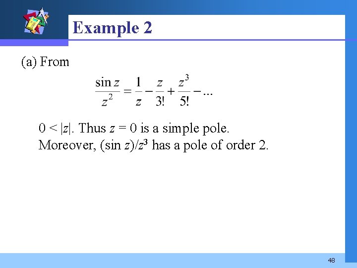
Example 2 (a) From 0 < |z|. Thus z = 0 is a simple pole. Moreover, (sin z)/z 3 has a pole of order 2. 48

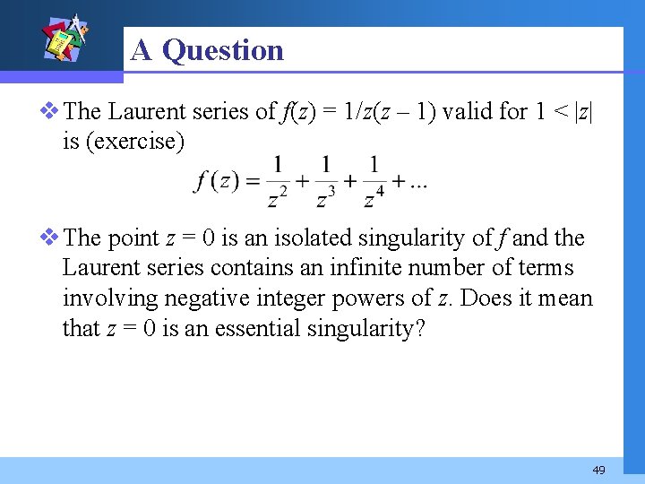
A Question v The Laurent series of f(z) = 1/z(z – 1) valid for 1 < |z| is (exercise) v The point z = 0 is an isolated singularity of f and the Laurent series contains an infinite number of terms involving negative integer powers of z. Does it mean that z = 0 is an essential singularity? 49

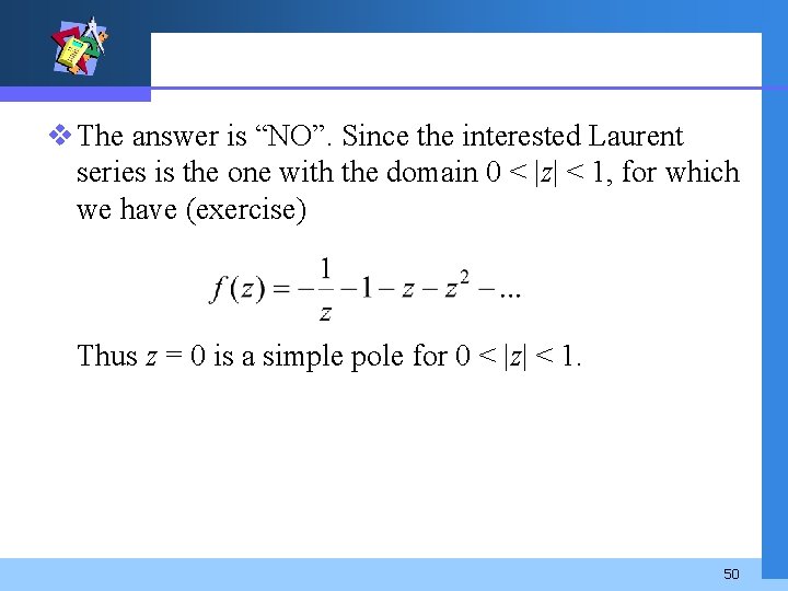
v The answer is “NO”. Since the interested Laurent series is the one with the domain 0 < |z| < 1, for which we have (exercise) Thus z = 0 is a simple pole for 0 < |z| < 1. 50

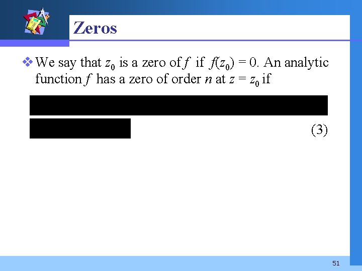
Zeros v We say that z 0 is a zero of f if f(z 0) = 0. An analytic function f has a zero of order n at z = z 0 if (3) 51

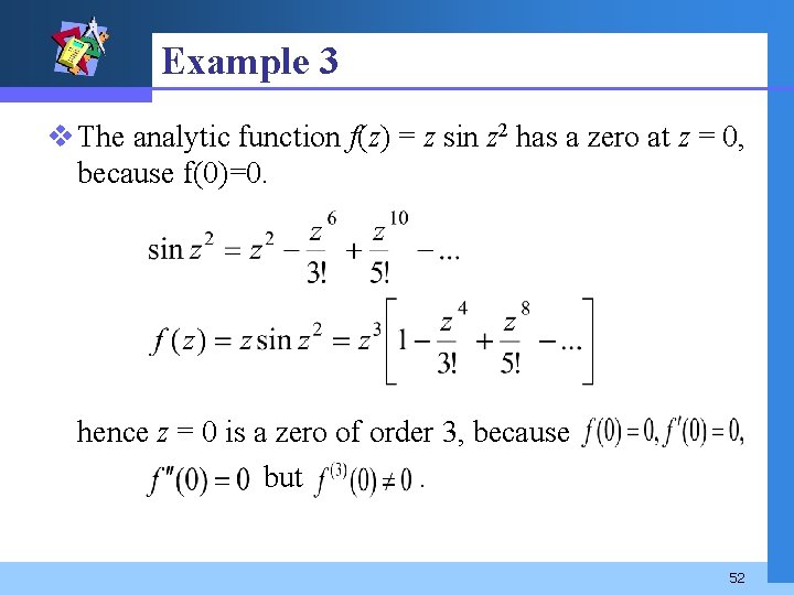
Example 3 v The analytic function f(z) = z sin z 2 has a zero at z = 0, because f(0)=0. hence z = 0 is a zero of order 3, because but. 52

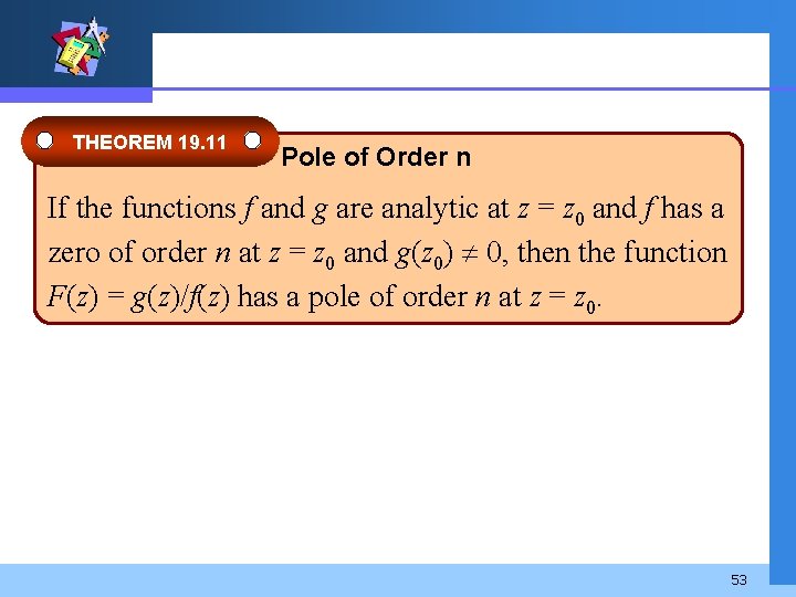
THEOREM 19. 11 Pole of Order n If the functions f and g are analytic at z = z 0 and f has a zero of order n at z = z 0 and g(z 0) 0, then the function F(z) = g(z)/f(z) has a pole of order n at z = z 0. 53

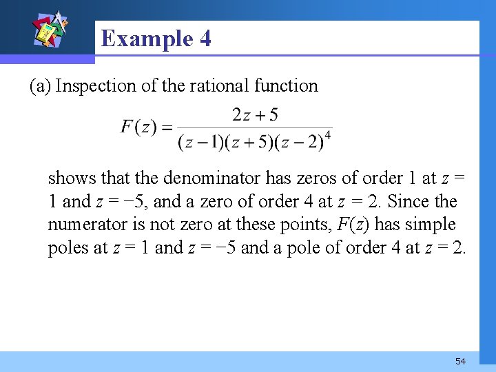
Example 4 (a) Inspection of the rational function shows that the denominator has zeros of order 1 at z = 1 and z = − 5, and a zero of order 4 at z = 2. Since the numerator is not zero at these points, F(z) has simple poles at z = 1 and z = − 5 and a pole of order 4 at z = 2. 54

19. 5 Residues and Residue Theorem v Residue The coefficient a-1 of 1/(z – z 0) in the Laurent series is called the residue of the function f at the isolated singularity. We use this notation a-1 = Res(f(z), z 0) 55

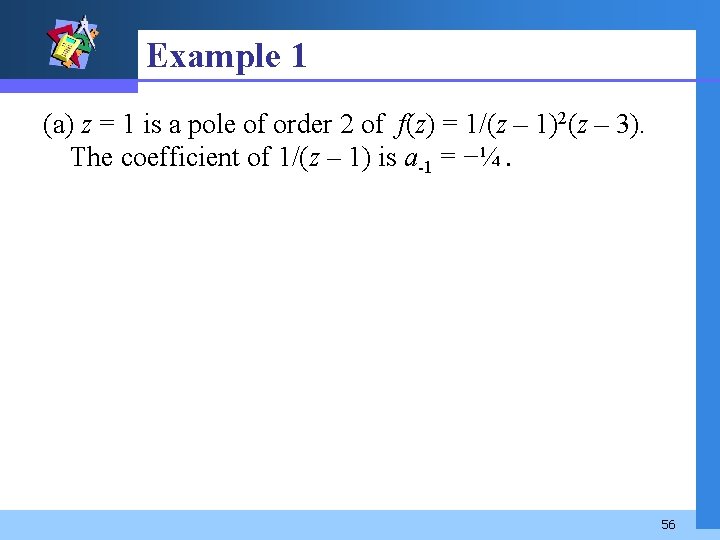
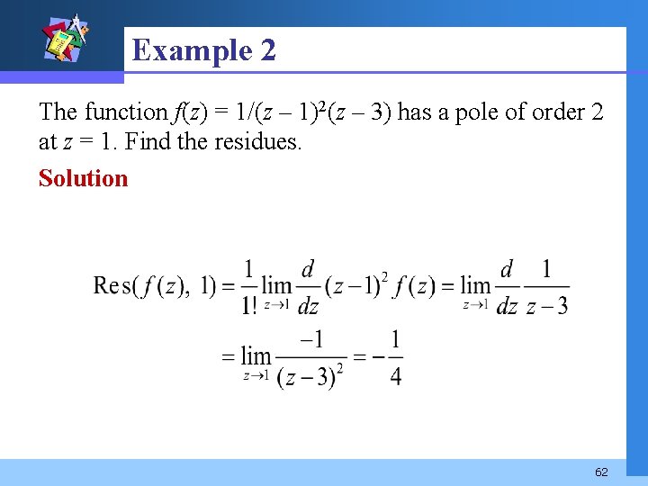
Example 1 (a) z = 1 is a pole of order 2 of f(z) = 1/(z – 1)2(z – 3). The coefficient of 1/(z – 1) is a-1 = −¼. 56

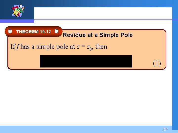
THEOREM 19. 12 Residue at a Simple Pole If f has a simple pole at z = z 0, then (1) 57

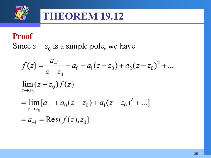
THEOREM 19. 12 Proof Since z = z 0 is a simple pole, we have 58

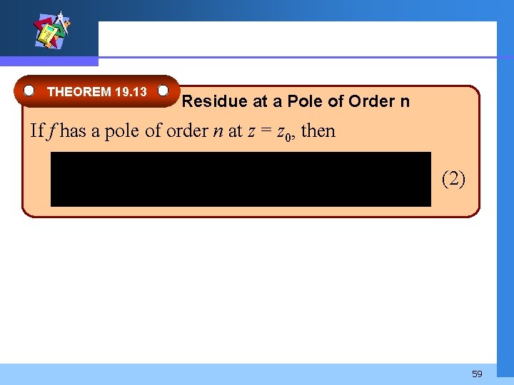
THEOREM 19. 13 Residue at a Pole of Order n If f has a pole of order n at z = z 0, then (2) 59

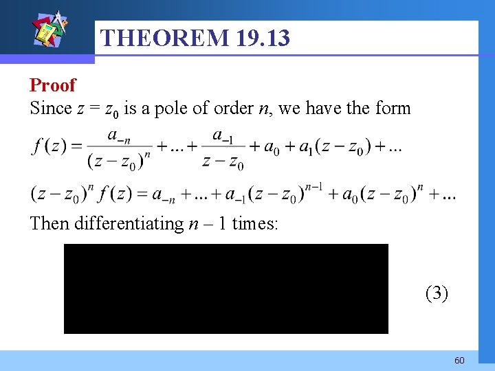
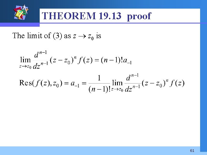
THEOREM 19. 13 Proof Since z = z 0 is a pole of order n, we have the form Then differentiating n – 1 times: (3) 60

THEOREM 19. 13 proof The limit of (3) as z z 0 is 61

Example 2 The function f(z) = 1/(z – 1)2(z – 3) has a pole of order 2 at z = 1. Find the residues. Solution 62

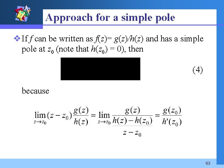
Approach for a simple pole v If f can be written as f(z)= g(z)/h(z) and has a simple pole at z 0 (note that h(z 0) = 0), then (4) because 63

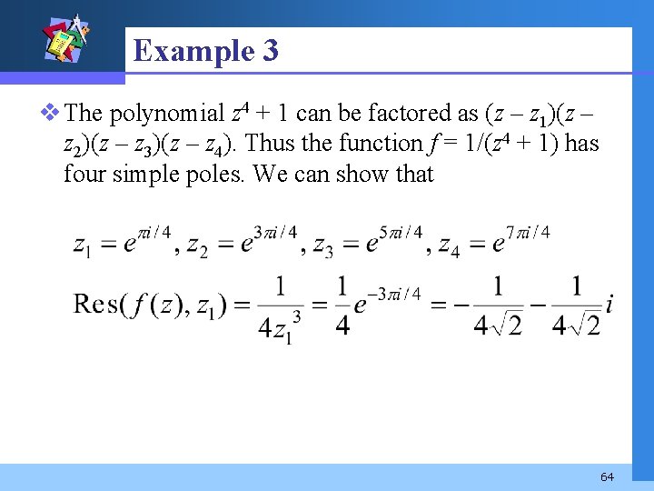
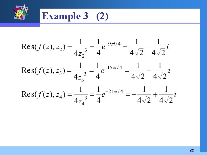
Example 3 v The polynomial z 4 + 1 can be factored as (z – z 1)(z – z 2)(z – z 3)(z – z 4). Thus the function f = 1/(z 4 + 1) has four simple poles. We can show that 64

Example 3 (2) 65

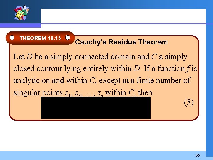
THEOREM 19. 15 Cauchy’s Residue Theorem Let D be a simply connected domain and C a simply closed contour lying entirely within D. If a function f is analytic on and within C, except at a finite number of singular points z 1, z 2, …, zn within C, then (5) 66

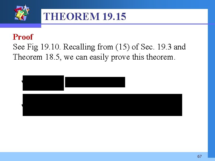
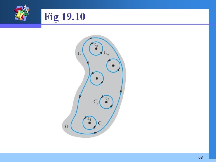
THEOREM 19. 15 Proof See Fig 19. 10. Recalling from (15) of Sec. 19. 3 and Theorem 18. 5, we can easily prove this theorem. 67

Fig 19. 10 68

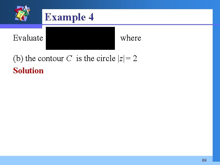
Example 4 Evaluate where (b) the contour C is the circle |z|= 2 Solution 69

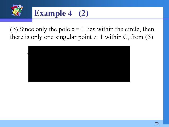
Example 4 (2) (b) Since only the pole z = 1 lies within the circle, then there is only one singular point z=1 within C, from (5) 70

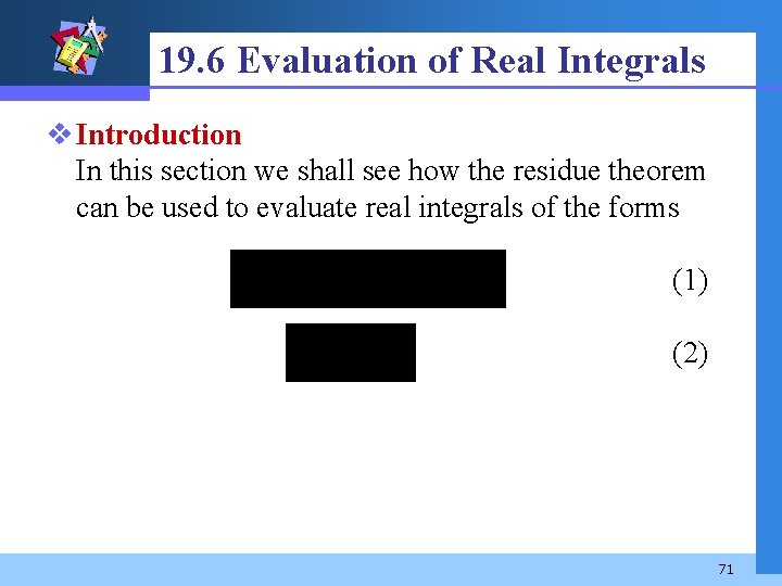
19. 6 Evaluation of Real Integrals v Introduction In this section we shall see how the residue theorem can be used to evaluate real integrals of the forms (1) (2) 71

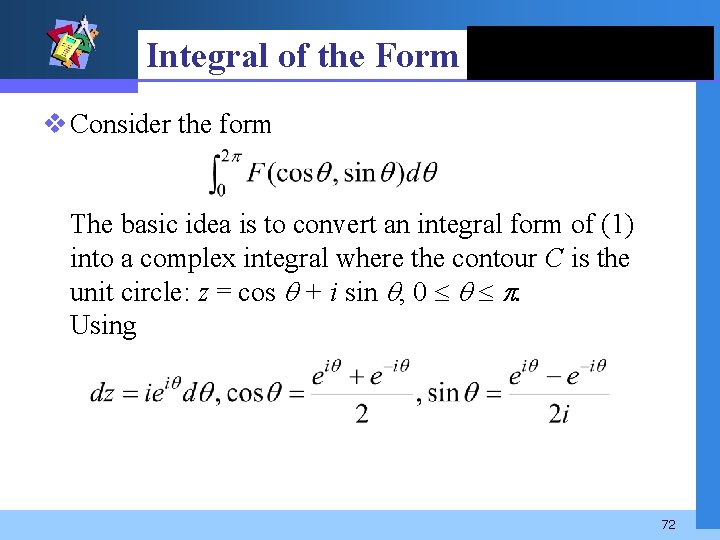
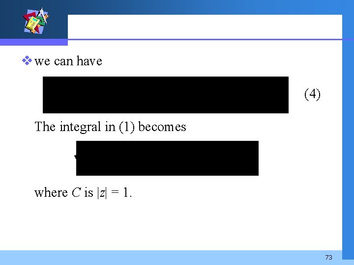
Integral of the Form v Consider the form The basic idea is to convert an integral form of (1) into a complex integral where the contour C is the unit circle: z = cos + i sin , 0 . Using 72

v we can have (4) The integral in (1) becomes where C is |z| = 1. 73

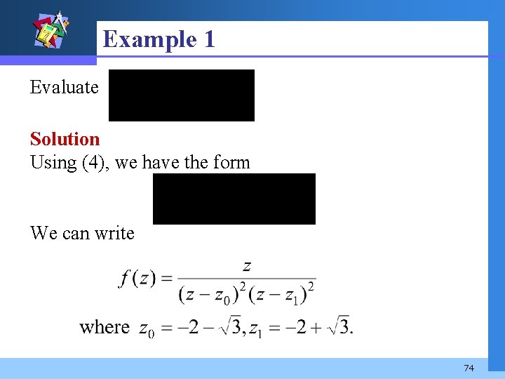
Example 1 Evaluate Solution Using (4), we have the form We can write 74

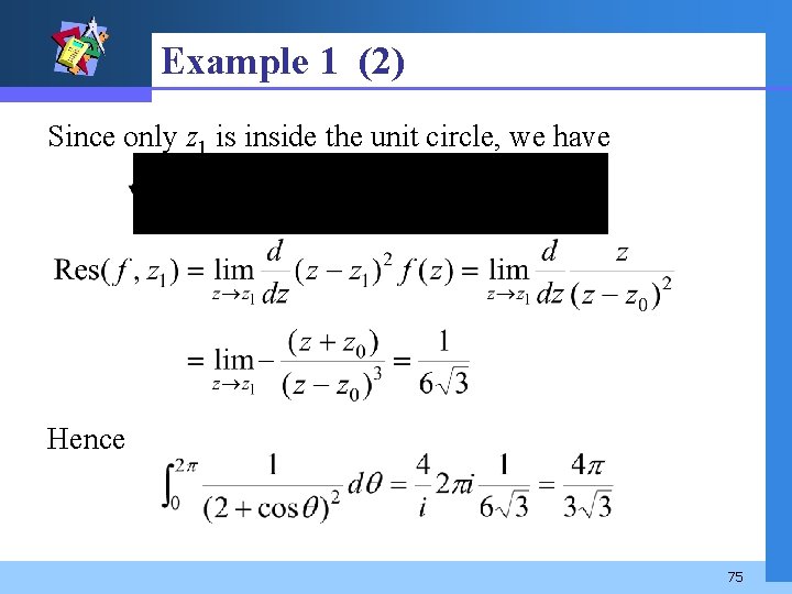
Example 1 (2) Since only z 1 is inside the unit circle, we have Hence 75

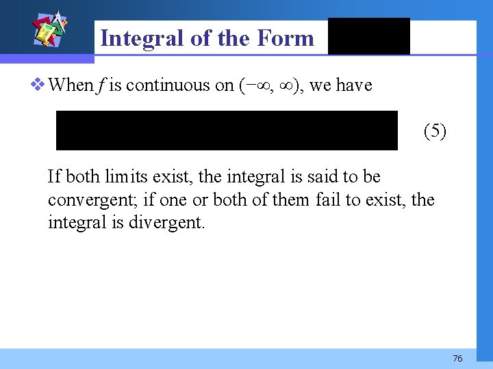
Integral of the Form v When f is continuous on (− , ), we have (5) If both limits exist, the integral is said to be convergent; if one or both of them fail to exist, the integral is divergent. 76

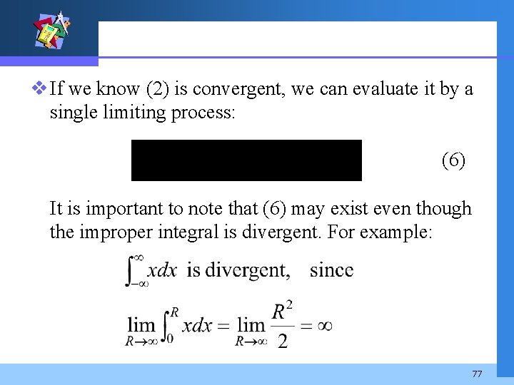
v If we know (2) is convergent, we can evaluate it by a single limiting process: (6) It is important to note that (6) may exist even though the improper integral is divergent. For example: 77

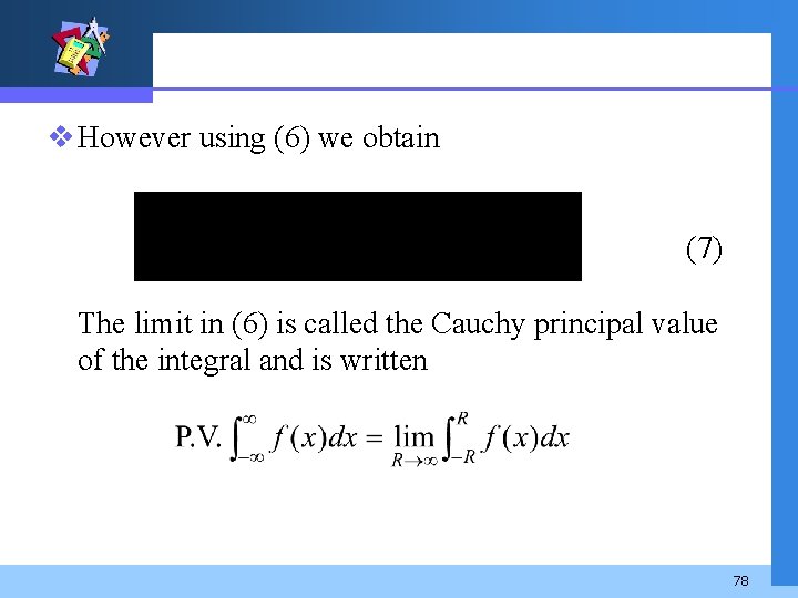
v However using (6) we obtain (7) The limit in (6) is called the Cauchy principal value of the integral and is written 78

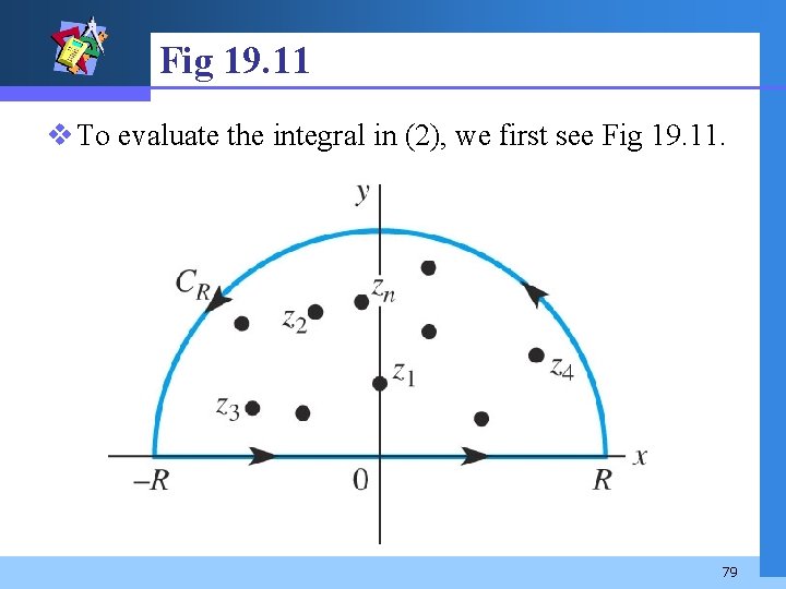
Fig 19. 11 v To evaluate the integral in (2), we first see Fig 19. 11. 79

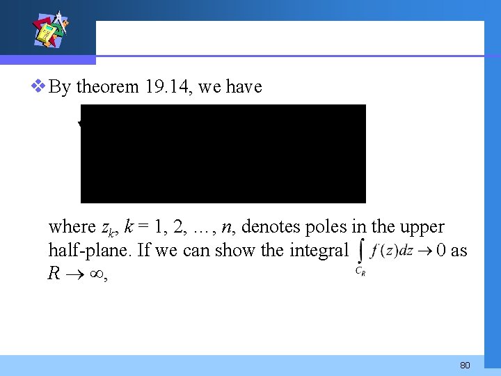
v By theorem 19. 14, we have where zk, k = 1, 2, …, n, denotes poles in the upper half-plane. If we can show the integral 0 as R , 80

then we have (8) 81

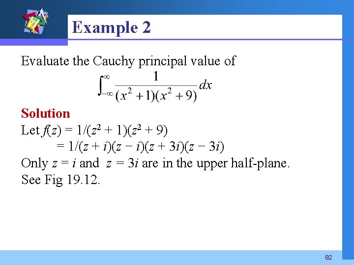
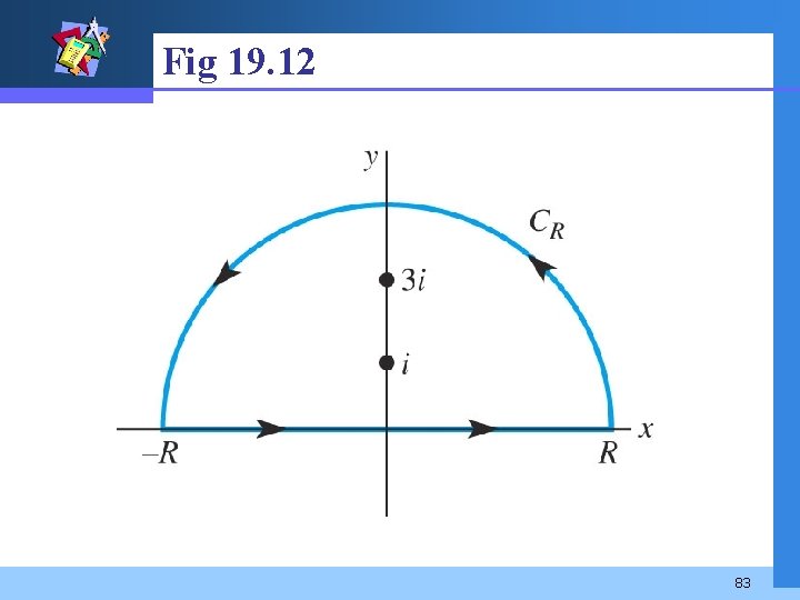
Example 2 Evaluate the Cauchy principal value of Solution Let f(z) = 1/(z 2 + 1)(z 2 + 9) = 1/(z + i)(z − i)(z + 3 i)(z − 3 i) Only z = i and z = 3 i are in the upper half-plane. See Fig 19. 12. 82

Fig 19. 12 83

Example 2 (2) (9) 84

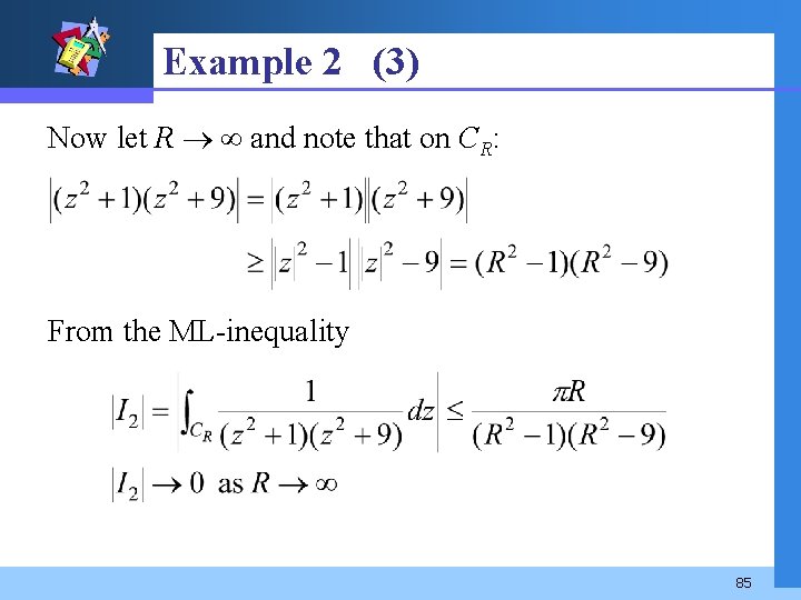
Example 2 (3) Now let R and note that on CR: From the ML-inequality 85

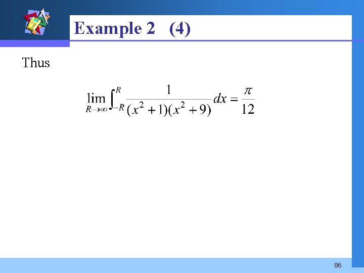
Example 2 (4) Thus 86

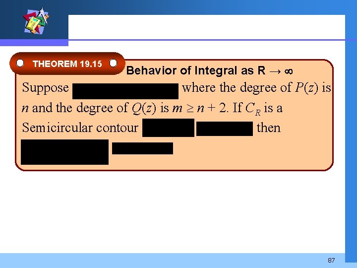
THEOREM 19. 15 Behavior of Integral as R → Suppose where the degree of P(z) is n and the degree of Q(z) is m n + 2. If CR is a Semicircular contour then 87

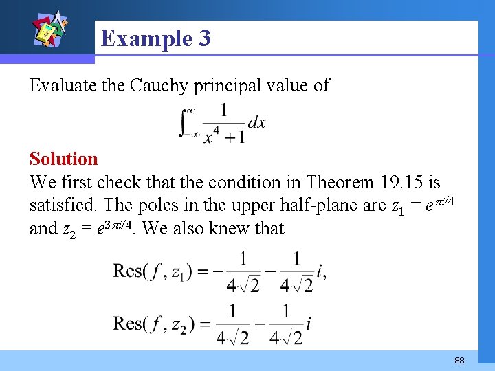
Example 3 Evaluate the Cauchy principal value of Solution We first check that the condition in Theorem 19. 15 is satisfied. The poles in the upper half-plane are z 1 = e i/4 and z 2 = e 3 i/4. We also knew that 88

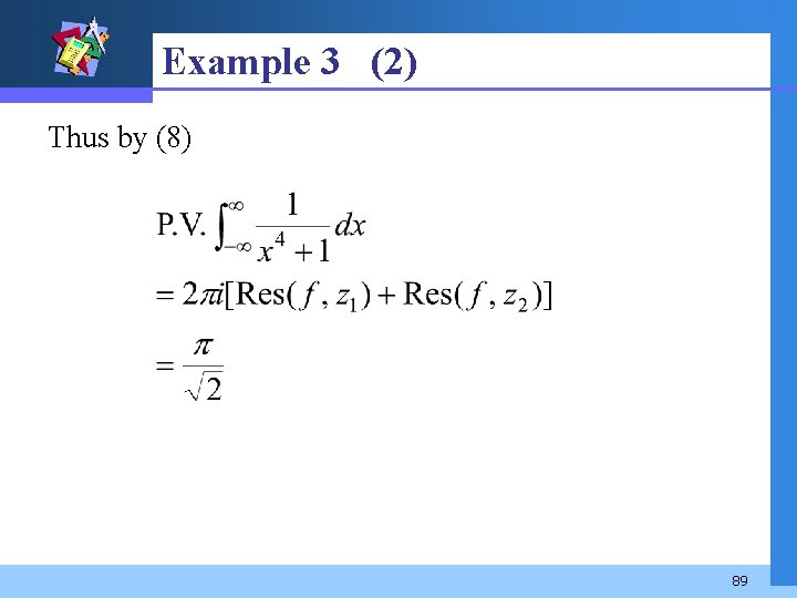
Example 3 (2) Thus by (8) 89

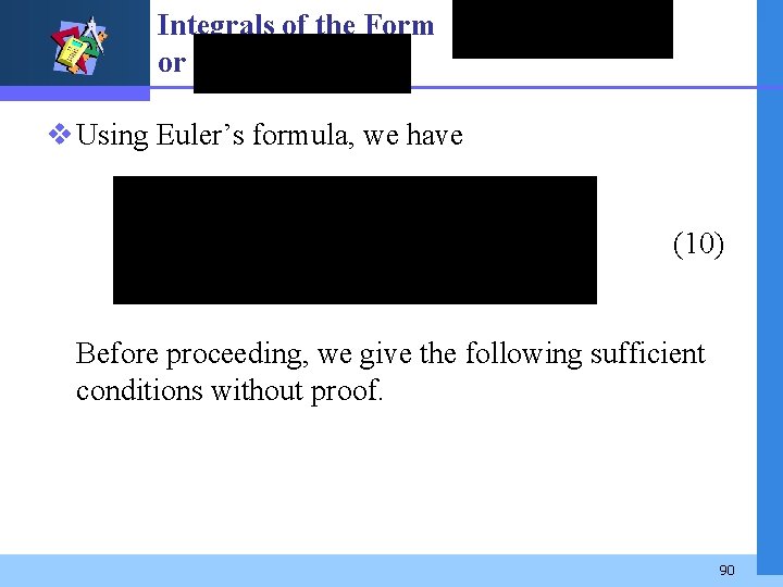
Integrals of the Form or v Using Euler’s formula, we have (10) Before proceeding, we give the following sufficient conditions without proof. 90

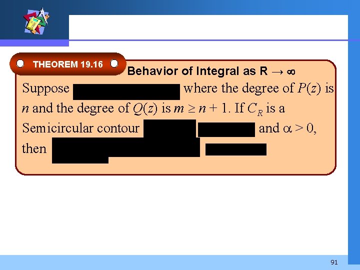
THEOREM 19. 16 Behavior of Integral as R → Suppose where the degree of P(z) is n and the degree of Q(z) is m n + 1. If CR is a Semicircular contour and > 0, then 91

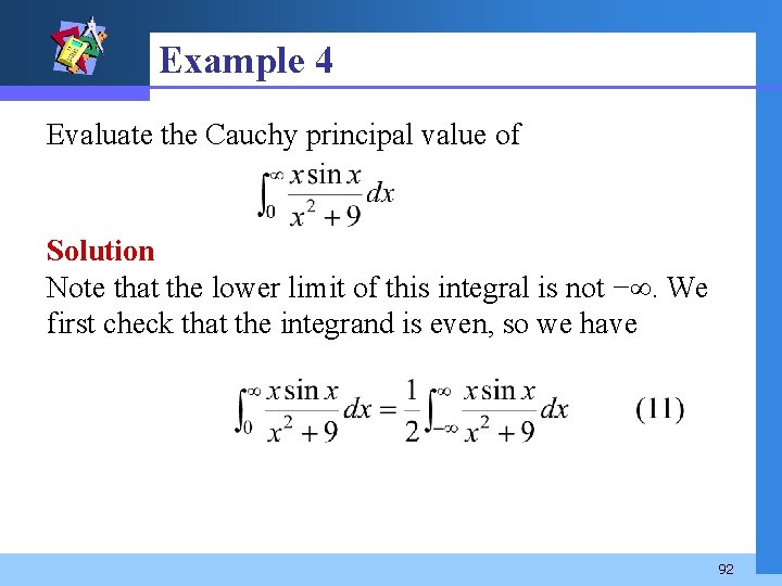
Example 4 Evaluate the Cauchy principal value of Solution Note that the lower limit of this integral is not −. We first check that the integrand is even, so we have 92

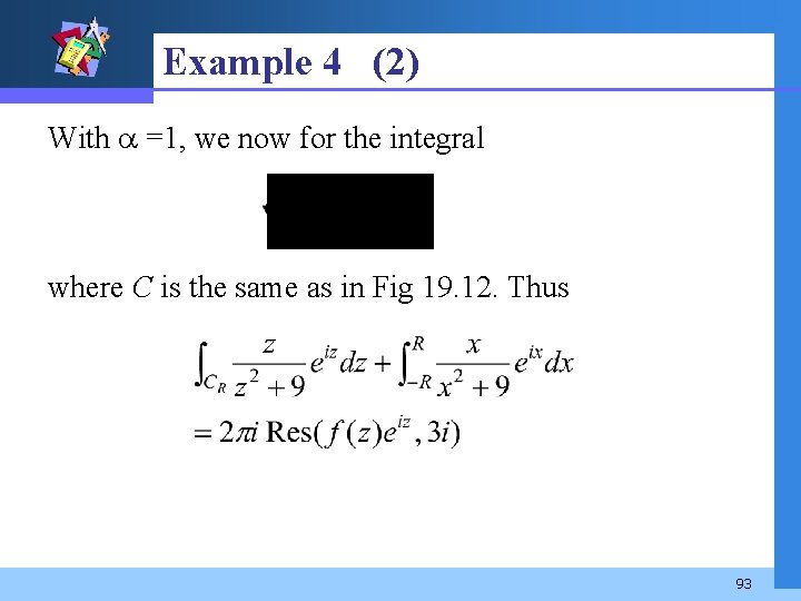
Example 4 (2) With =1, we now for the integral where C is the same as in Fig 19. 12. Thus 93

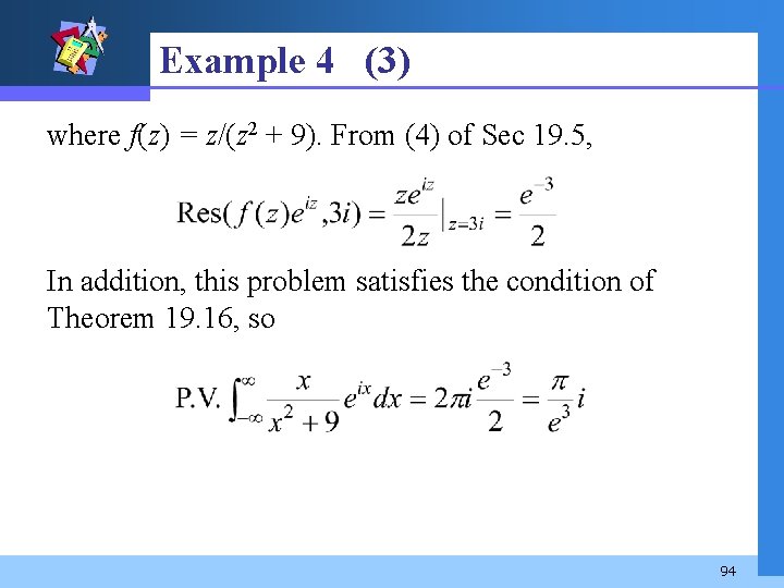
Example 4 (3) where f(z) = z/(z 2 + 9). From (4) of Sec 19. 5, In addition, this problem satisfies the condition of Theorem 19. 16, so 94

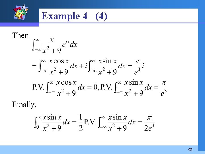
Example 4 (4) Then Finally, 95

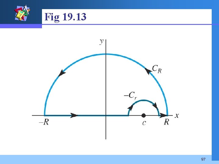
Indented Contour v The complex functions f(z) = P(z)/Q(z) of the improper integrals (2) and (3) did not have poles on the real axis. When f(z) has a pole at z = c, where c is a real number, we must use the indented contour as in Fig 19. 13. 96

Fig 19. 13 97

THEOREM 19. 17 Behavior of Integral as r → Suppose f has a simple pole z = c on the real axis. If Cr is the contour defined by 98

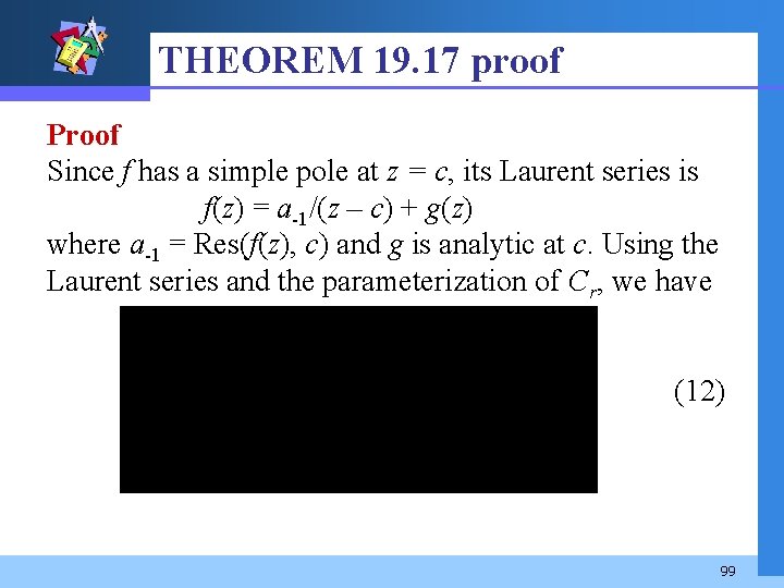
THEOREM 19. 17 proof Proof Since f has a simple pole at z = c, its Laurent series is f(z) = a-1/(z – c) + g(z) where a-1 = Res(f(z), c) and g is analytic at c. Using the Laurent series and the parameterization of Cr, we have (12) 99

THEOREM 19. 17 proof First we see Next, g is analytic at c and so it is continuous at c and is bounded in a neighborhood of the point; that is, there exists an M > 0 for which |g(c + rei )| M. Hence It follows that limr 0|I 2| = 0 and limr 0 I 2 = 0. We complete the proof. 100

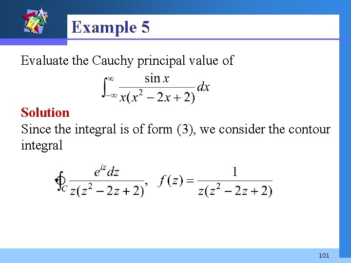
Example 5 Evaluate the Cauchy principal value of Solution Since the integral is of form (3), we consider the contour integral 101

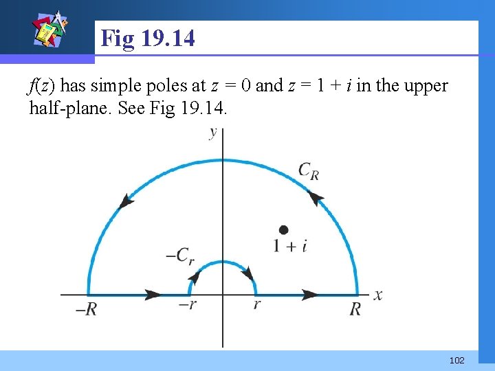
Fig 19. 14 f(z) has simple poles at z = 0 and z = 1 + i in the upper half-plane. See Fig 19. 14. 102

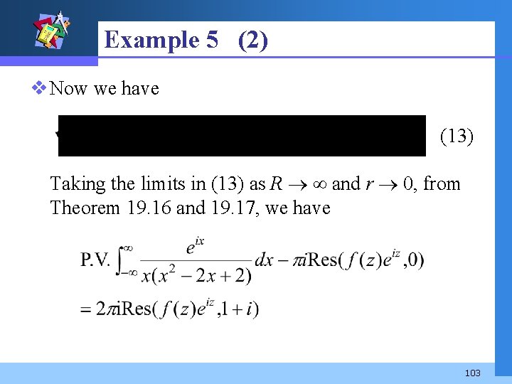
Example 5 (2) v Now we have (13) Taking the limits in (13) as R and r 0, from Theorem 19. 16 and 19. 17, we have 103

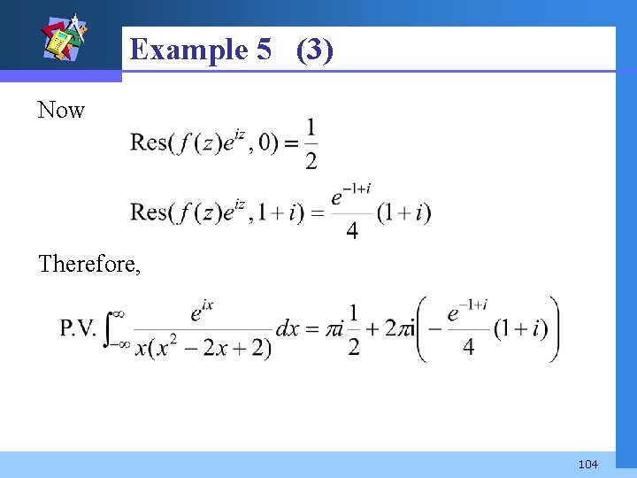
Example 5 (3) Now Therefore, 104

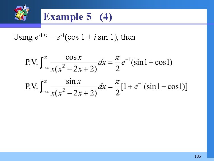
Example 5 (4) Using e-1+i = e-1(cos 1 + i sin 1), then 105