Chapter 13 Simple Linear Regression and Correlation Inferential

Chapter 13 Simple Linear Regression and Correlation: Inferential Methods

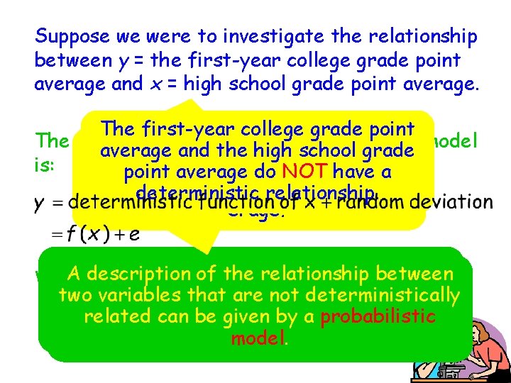
Suppose we were to investigate the relationship between y = the first-year college grade point average and x = high school grade point average. The first-year college grade point The equation anthe additive probabilistic Is thefor first-year college grade average and high school grade model is: point average determined point average do NOT solely have aby the high school relationship. grade point deterministic average? A description relationshipof in the which the value of y is A relationship between Where e is an determined “error” variable completely by the value of an two variables that are not deterministically independent called a related can bevariable given byxaisprobabilistic deterministic relationship. model.

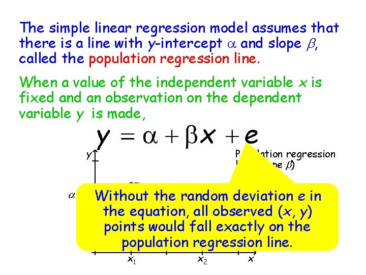
The simple linear regression model assumes that there is a line with y-intercept a and slope b, called the population regression line. When a value of the independent variable x is fixed an observation on the dependent variable y is made, y a Population regression line (slope b) e 1 Without the random deviation e in e 2 the equation, all observed (x, y) points would fall exactly on the population regression line. x 1 x 2 x

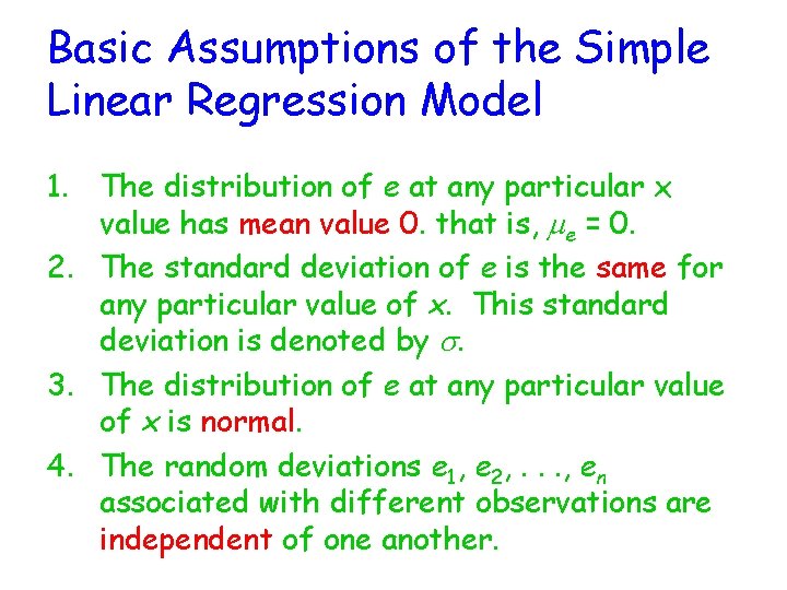
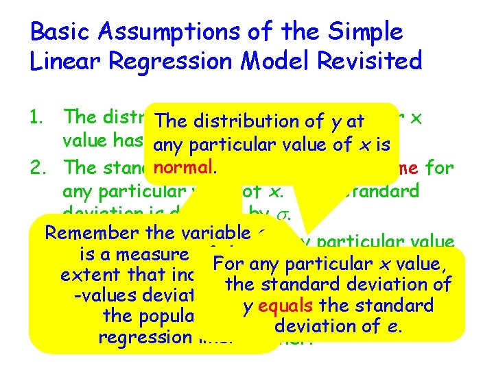
Basic Assumptions of the Simple Linear Regression Model 1. The distribution of e at any particular x value has mean value 0. that is, me = 0. 2. The standard deviation of e is the same for any particular value of x. This standard deviation is denoted by s. 3. The distribution of e at any particular value of x is normal. 4. The random deviations e 1, e 2, . . . , en associated with different observations are independent of one another.

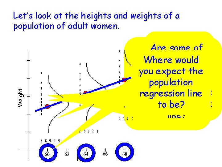
Let’s look at the heights and weights of a population of adult women. Weight How much Weights women Are of some of would an that. We are 5 feet tall want these weights Where would adult What would will vary – infemale other standard This distribution more likelyisthe than you expect words, there a weigh if she you expect deviations of all ispopulation normally others? distribution of were 5 feet for other thesefor normal distributed. What would this weights adult regression line tall? heights? females 5 to distributions distribution towho be? are look feet tall. be the same. like? Height

Basic Assumptions of the Simple Linear Regression Model Revisited 1. The distribution of e at anyofparticular x The distribution y at value has mean value 0. that any particular valueis, ofmex=is 0. normal. 2. The standard deviation of e is the same for any particular value of x. This standard deviation is denoted by s. the variable e any particular value 3. Remember The distribution of e at is a measure of the of x is normal. For any particular x value, extent that individual y the standard deviation of 4. The random deviations e , . . . , e -values deviate from 1 2 n y equals the standard associated with different observations are the population deviation of e. regression independent ofline. one another.

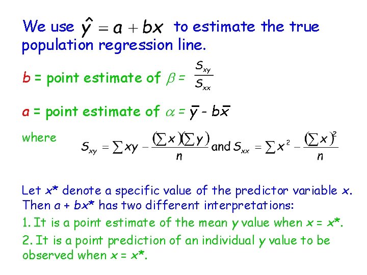
We use to estimate the true population regression line. b = point estimate of b = a = point estimate of a = y - bx where Let x* denote a specific value of the predictor variable x. Then a + bx* has two different interpretations: 1. It is a point estimate of the mean y value when x = x*. 2. It is a point prediction of an individual y value to be observed when x = x*.

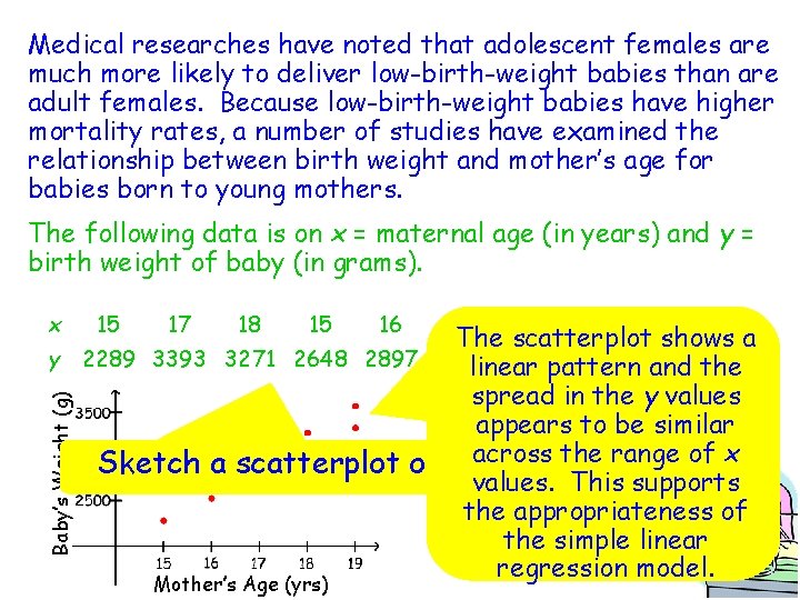
Medical researches have noted that adolescent females are much more likely to deliver low-birth-weight babies than are adult females. Because low-birth-weight babies have higher mortality rates, a number of studies have examined the relationship between birth weight and mother’s age for babies born to young mothers. The following data is on x = maternal age (in years) and y = birth weight of baby (in grams). x 15 17 18 15 16 19 17 16 18 19 Baby’s Weight (g) The scatterplot shows a y 2289 3393 3271 2648 2897 3327 2970 2535 3138 3573 linear pattern and the spread in the y values appears to be similar acrossdata. the range of x Sketch a scatterplot of these values. This supports the appropriateness of the simple linear regression model. Mother’s Age (yrs)

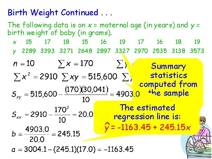
Birth Weight Continued. . . The following data is on x = maternal age (in years) and y = birth weight of baby (in grams). x 15 17 18 15 16 19 17 16 18 19 y 2289 3393 3271 2648 2897 3327 2970 2535 3138 3573 Summary statistics computed from the sample datathese are: Using The estimated summary regression line is: statistics y = -1163. 45 + 245. 15 x

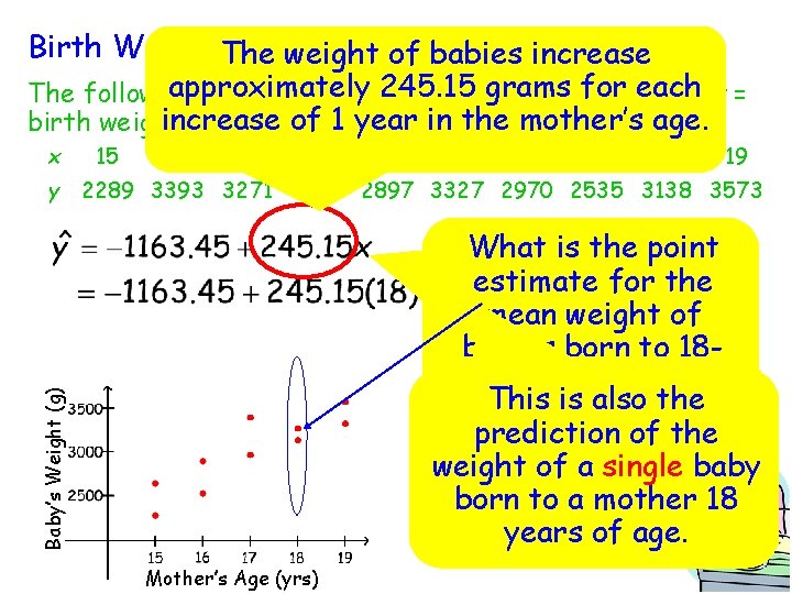
Birth Weight The Continued. . babies increase weight. of approximately 245. 15 grams for each The following data is on x = maternal age (in years) and y = increase of grams). 1 year in the mother’s age. birth weight of baby (in x 15 17 18 15 16 19 17 16 18 19 y 2289 3393 3271 2648 2897 3327 2970 2535 3138 3573 Baby’s Weight (g) What is the point estimate for the mean weight of babies born to 18 year-old mothers? This is the This is alsopoint the estimate for the prediction of the meanof weight of baby all weight a single babies to 18 born to aborn mother 18 year-old mothers. years of age. Mother’s Age (yrs)

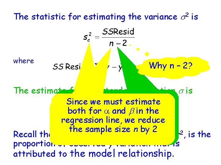
The statistic for estimating the variance s 2 is where Why n – 2? The estimate for the standard deviation s is Note the degrees Since that we must estimateof freedom associated with The subscript e reminds us both for a and b in the 2 or s in simple estimating s that we are estimating the regression line, we reduce variance of regression the “errors” thelinear sample size n byis 2 or 2, is the Recall the coefficient of determination, r residuals. df = n - 2 proportion of observed y variation that is attributed to the model relationship.

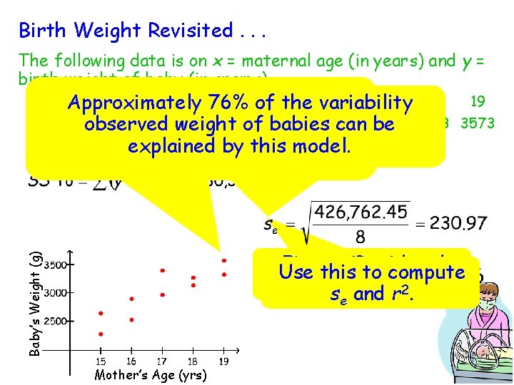
Birth Weight Revisited. . . The following data is on x = maternal age (in years) and y = birth weight of baby (in grams). For a particular mother’s age, the 15 17 18 1576%16 of the 19 variability 17 16 18 Approximately typical y 2289 3393 deviation 3271 weight 2648 for 2897 3327 2970 observed ofpossible babies can 2535 be 3138 weights ofexplained babies isby approximately this model. 231 grams. x 19 3573 Baby’s Weight (g) Findthis SSResid and Use to compute 2. s. SSTo. and r e Mother’s Age (yrs)

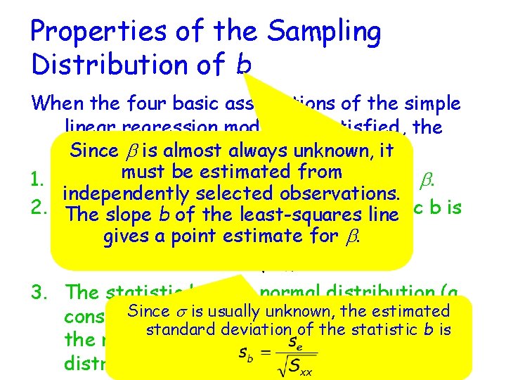
Properties of the Sampling Distribution of b When the four basic assumptions of the simple linear regression model are satisfied, the Since b isstatements almost always it following are unknown, true: mustvalue be estimated 1. The mean of b is b. from That is, mb = b. independently selected observations. 2. The slope standard of the statistic b is b ofdeviation the least-squares line gives a point estimate for b. 3. The statistic b has a normal distribution (a Since sof is usually unknown, the estimated consequence the model assumption that standard deviation of the statistic b is the random deviation e is normally distributed. )

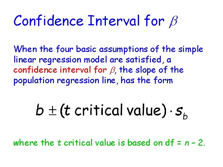
Confidence Interval for b When the four basic assumptions of the simple linear regression model are satisfied, a confidence interval for b, the slope of the population regression line, has the form where the t critical value is based on df = n – 2.

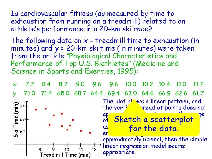
Is cardiovascular fitness (as measured by time to exhaustion from running on a treadmill) related to an athlete’s performance in a 20 -km ski race? The following data on x = treadmill time to exhaustion (in minutes) and y = 20 -km ski time (in minutes) were taken from the article “Physiological Characteristics and Performance of Top U. S. Biathletes” (Medicine and Science in Sports and Exercise, 1995): 7. 7 y 71. 0 71. 4 65. 0 68. 7 64. 4 69. 4 63. 0 64. 6 66. 9 62. 6 61. 7 The plot shows a linear pattern, and the vertical spread of points does not appear to be changing over the range a scatterplot of x. Sketch values in the sample. If we assume that the distribution of for the data. errors at any given x value is approximately normal, then the simple linear regression model seems appropriate. Treadmill Time (min) Ski Time (min) x 8. 4 8. 7 9. 0 9. 6 10. 0 10. 2 10. 4 11. 0 11. 7

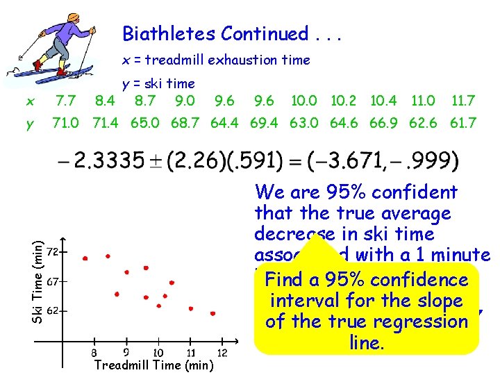
Biathletes Continued. . . x = treadmill exhaustion time y = ski time 8. 4 8. 7 9. 0 x 7. 7 9. 6 10. 0 10. 2 10. 4 11. 0 11. 7 y 71. 0 71. 4 65. 0 68. 7 64. 4 69. 4 63. 0 64. 6 66. 9 62. 6 61. 7 Ski Time (min) We are 95% confident that the true average decrease in ski time associated with a 1 minute increase in treadmill Find a 95% confidence exhaustion time interval for theisslope between 1 minute and 3. 7 of the true regression minutes. line. Treadmill Time (min)

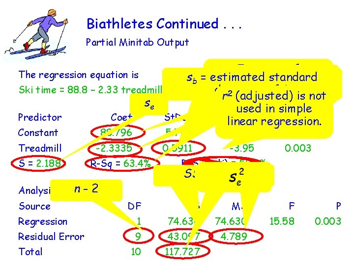
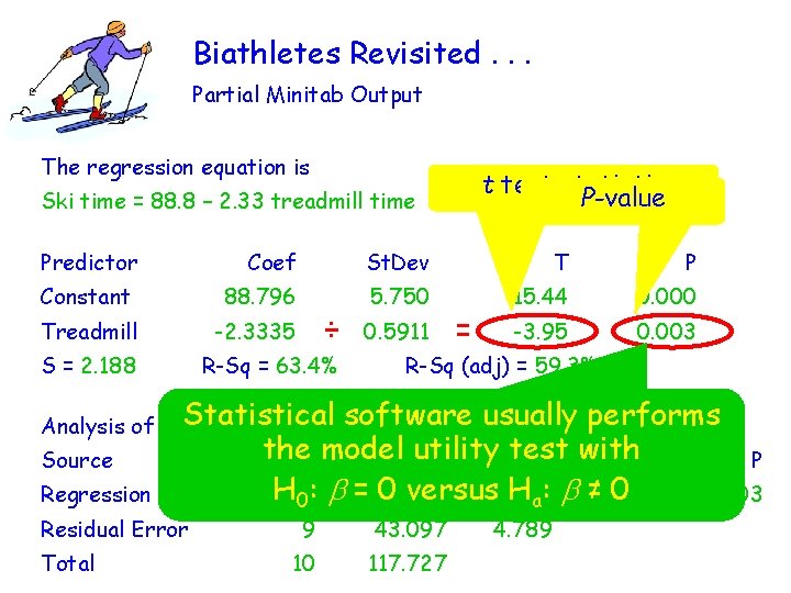
Biathletes Continued. . . Partial Minitab Output Equation of y Estimated sb = estimated standard estimated regression intercept a b Ski time = 88. 8 – 2. 33 treadmill time deviation of b Estimated slope 2 line r 100×r (adjusted) is not 2 se used in simple Predictor Coef St. Dev T regression. P linear The regression equation is Constant 88. 796 5. 750 15. 44 0. 000 Treadmill -2. 3335 0. 5911 -3. 95 0. 003 S = 2. 188 R-Sq = 63. 4% n-2 Analysis of Variance Source R-Sq (adj) = 59. 3% SSResid SSTo DF SS MS F P Regression 1 74. 630 15. 58 0. 003 Residual Error 9 43. 097 4. 789 10 117. 727 Total

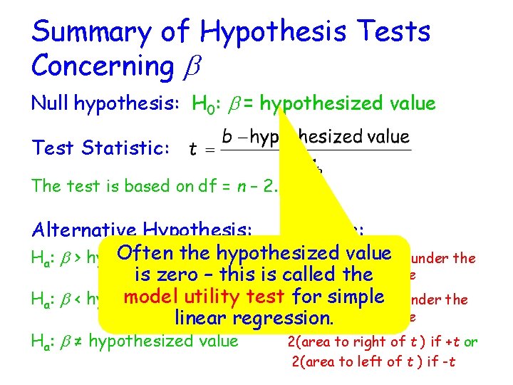
Summary of Hypothesis Tests Concerning b Null hypothesis: H 0: b = hypothesized value Test Statistic: The test is based on df = n – 2. Alternative Hypothesis: P -value: Often the hypothesized value Ha: b > hypothesized value area to right of t under the appropriate is zero – this is called thet curve model utility fortosimple Ha: b < hypothesized value test area left of t under the appropriate t curve linear regression. Ha: b ≠ hypothesized value 2(area to right of t ) if +t or 2(area to left of t ) if -t

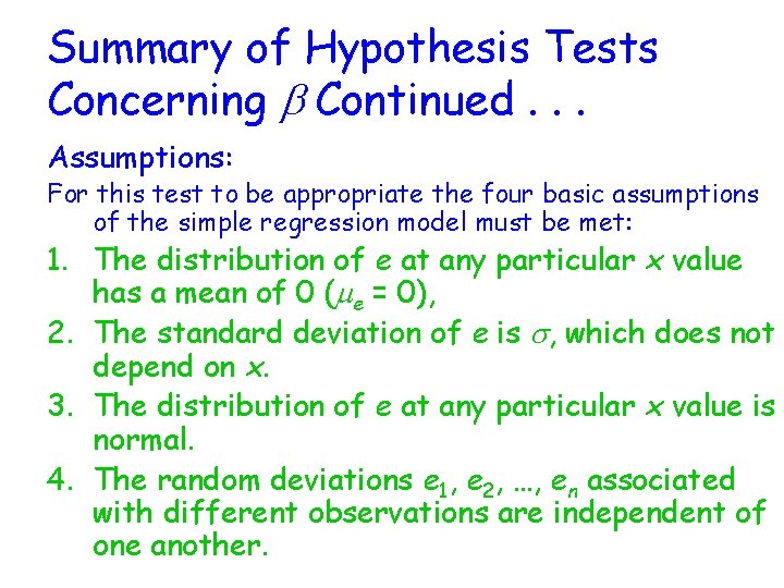
Summary of Hypothesis Tests Concerning b Continued. . . Assumptions: For this test to be appropriate the four basic assumptions of the simple regression model must be met: 1. The distribution of e at any particular x value has a mean of 0 (me = 0), 2. The standard deviation of e is s, which does not depend on x. 3. The distribution of e at any particular x value is normal. 4. The random deviations e 1, e 2, …, en associated with different observations are independent of one another.

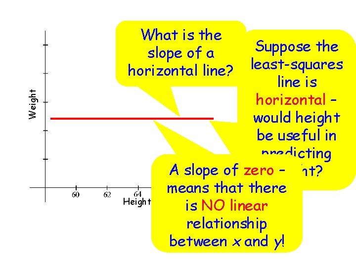
Weight What is the slope of a horizontal line? Height Suppose the least-squares line is horizontal – would height be useful in predicting A slope of zeroweight? – means that there is NO linear relationship between x and y!

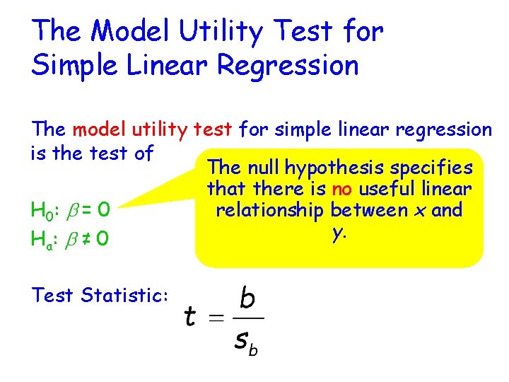
The Model Utility Test for Simple Linear Regression The model utility test for simple linear regression is the test of The null hypothesis specifies that there is no useful linear relationship between x and H 0 : b = 0 y. Ha : b ≠ 0 Test Statistic:

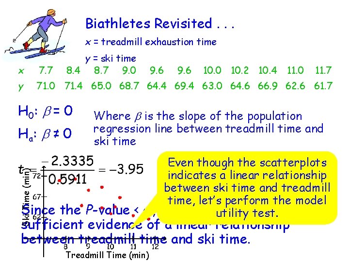
Biathletes Revisited. . . x = treadmill exhaustion time y = ski time 8. 4 8. 7 9. 0 x 7. 7 y 71. 0 71. 4 65. 0 68. 7 64. 4 69. 4 63. 0 64. 6 66. 9 62. 6 61. 7 H 0 : b = 0 Ha : b ≠ 0 9. 6 10. 0 10. 2 10. 4 11. 0 11. 7 Where b is the slope of the population regression line between treadmill time and ski time Ski Time (min) P-value = the. 003 scatterplots Even though indicates a linear relationship a =. 05 df = 9 between ski time and treadmill time, let’s perform the model Since the P-value < a, we rejectutility H 0. There test. is sufficient evidence of a linear relationship between treadmill time and ski time. Treadmill Time (min)

Biathletes Revisited. . . Partial Minitab Output The regression equation is t test statistic P-value Ski time = 88. 8 – 2. 33 treadmill time Predictor Coef St. Dev T P Constant 88. 796 5. 750 15. 44 0. 000 Treadmill -2. 3335 -3. 95 0. 003 S = 2. 188 ÷ R-Sq = 63. 4% 0. 5911 = R-Sq (adj) = 59. 3% Statistical Analysis of Variance Source Regression Residual Error Total software usually performs the test DF model utility SS MS with F P H 01: b = 74. 630 0 versus Ha: b ≠ 15. 58 0 74. 630 0. 003 9 43. 097 10 117. 727 4. 789

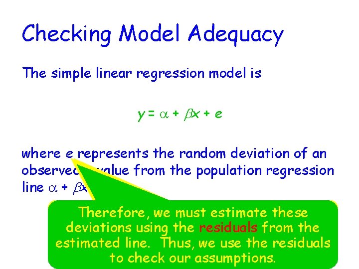
Checking Model Adequacy The simple linear regression model is y = a + bx + e where e represents the random deviation of an observed y value from the population regression line a + bx. If However, we knew we the do deviations not know the of edeviations ethese Therefore, we must 1, linear 2, …, en, The assumptions forestimate simple for we e 1, e could examine en because them for population any the deviations using the residuals from 2, …, regression are based onthe this random inconsistencies regression with linemodel is e. unknown. assumptions. estimated line. deviation Thus, we use the residuals to check our assumptions.

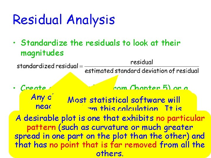
Residual Analysis • Standardize the residuals to look at their magnitudes • Create a residual plot (from Chapter 5) or a Any observation with a large positive or of standardized residual plot (which is a plot Most statistical software will residualthis should bepairs) examined the negative (x, standardized residual) perform calculation. It is carefullyplot for is any error recording tedious toinexhibits do by hand. A desirable one that no data, particular nonstandard experimental condition, or pattern (such as curvature or much greater atypical experimental unit. spread in one part on the plot than the other) and that has no point that is far removed from all the others.

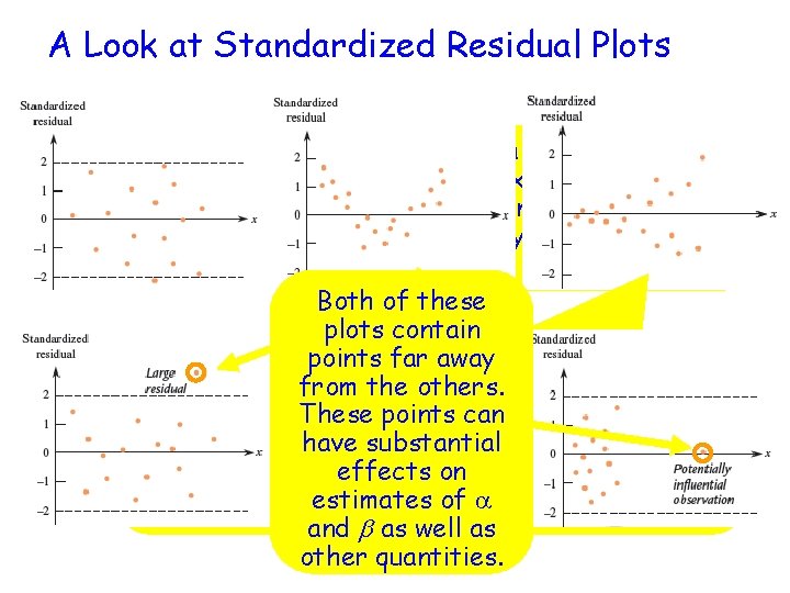
A Look at Standardized Residual Plots This is a desirable plot in that it exhibits no pattern and has no point that lies far away from the other points. Both of these plots contain points farplot away This exhibits a curved In this plot, the standard deviation of the frompattern the others. which indicates that residuals increases as thecan x-values increase. Thesethe points fitted model should be While a straight-line model might still be have changed substantial to incorporate the appropriate, the best-fit should be found effects online curvature. using weightedestimates least-squares. of a Consult your local statistician! and b as well as other quantities.

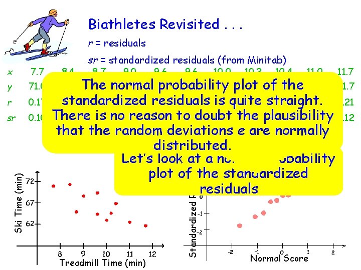
Biathletes Revisited. . . r = residuals y 71. 0 r 0. 17 sr 0. 10 8. 4 8. 7 9. 0 9. 6 10. 0 10. 2 10. 4 11. 0 11. 7 The probability the 62. 6 61. 7 65. 0 normal 68. 7 64. 4 69. 4 63. 0 plot 64. 6 of 66. 9 standardized residuals is quite 2. 21 -3. 49 0. 91 -1. 99 3. 01 -2. 46 -0. 39 straight. 2. 37 -0. 53 0. 21 There is no 0. 44 reason doubt 1. 13 -1. 74 -0. 96 to 1. 44 -1. 18 the -0. 19 plausibility 1. 16 -0. 27 0. 12 that the random deviations e are normally distributed. Let’s look at a normal probability plot of the standardized residuals 71. 4 Treadmill Time (min) Standardized Residual 7. 7 Ski Time (min) x sr = standardized residuals (from Minitab) Normal Score

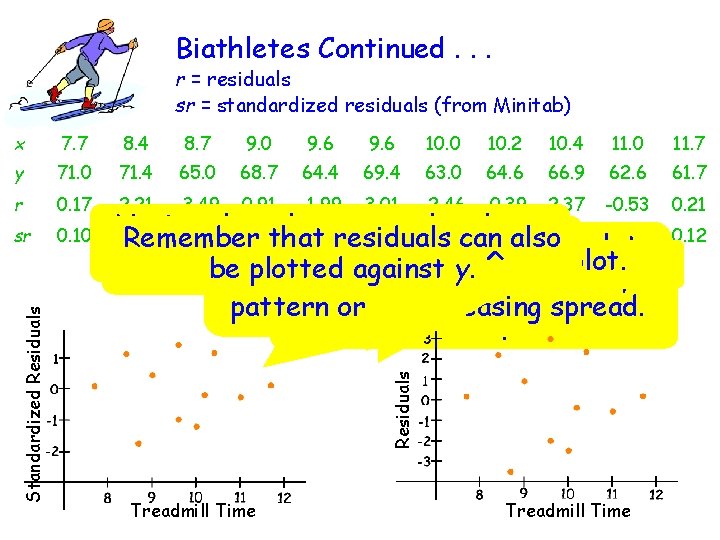
Biathletes Continued. . . r = residuals sr = standardized residuals (from Minitab) 7. 7 8. 4 8. 7 9. 0 9. 6 10. 0 10. 2 10. 4 11. 0 11. 7 y 71. 0 71. 4 65. 0 68. 7 64. 4 69. 4 63. 0 64. 6 66. 9 62. 6 61. 7 r 0. 17 2. 21 -3. 49 0. 91 -1. 99 3. 01 -2. 46 -0. 39 2. 37 -0. 53 0. 21 sr 0. 10 Notice these two have 1. 13 -1. 74 that 0. 44 -0. 96 1. 44 plots -1. 18 can -0. 19 -0. 27 Remember that residuals also 1. 16 plot The standardized residual similar appearances. Sketch a y. residual plot. bedoes plotted against not show evidence of any Sketch a standardized pattern or of increasing spread. residual plot. Residuals Standardized Residuals x Treadmill Time 0. 12

Optional Topics Inferences Based on the Estimated Regression Line and Inference about the Population Correlation Coefficient

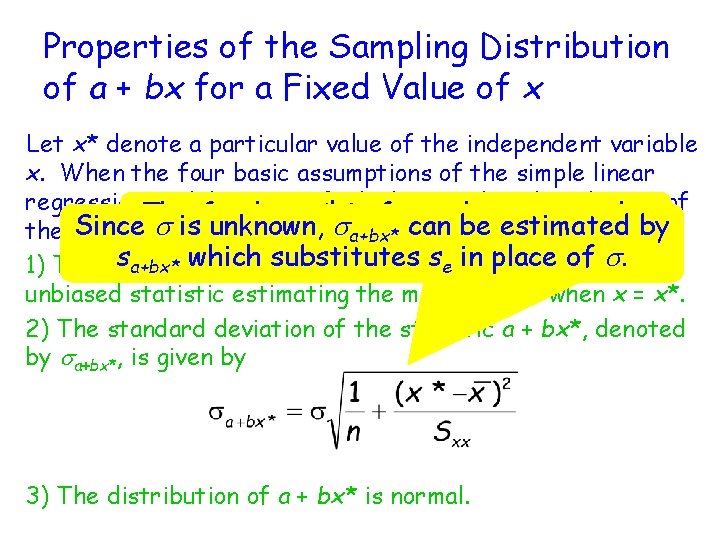
Properties of the Sampling Distribution of a + bx for a Fixed Value of x Let x* denote a particular value of the independent variable x. When the four basic assumptions of the simple linear regression model are satisfied, the sampling distribution of The farther x*sis from the center, theby Since s is unknown, can be estimated the statistic a +bx* had the following properties: a+bx* larger sa+bx* is. place of s. s which substitutes s in a+bx* e so a + bx* is an 1) The mean value of a + bx* is a + bx*, unbiased statistic estimating the mean y value when x = x*. 2) The standard deviation of the statistic a + bx*, denoted by sa+bx*, is given by 3) The distribution of a + bx* is normal.

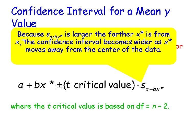
Confidence Interval for a Mean y Value Because s is larger the farther x* is from a+bx* When the basic assumptions of the simple linear x, the confidence interval becomes wider as x* regression modelfrom are met, a confidence moves away the center of the interval data. for a +bx*, the mean y value when x has value x*, is where the t critical value is based on df = n – 2.

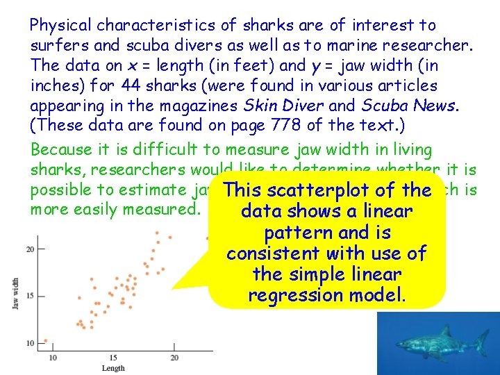
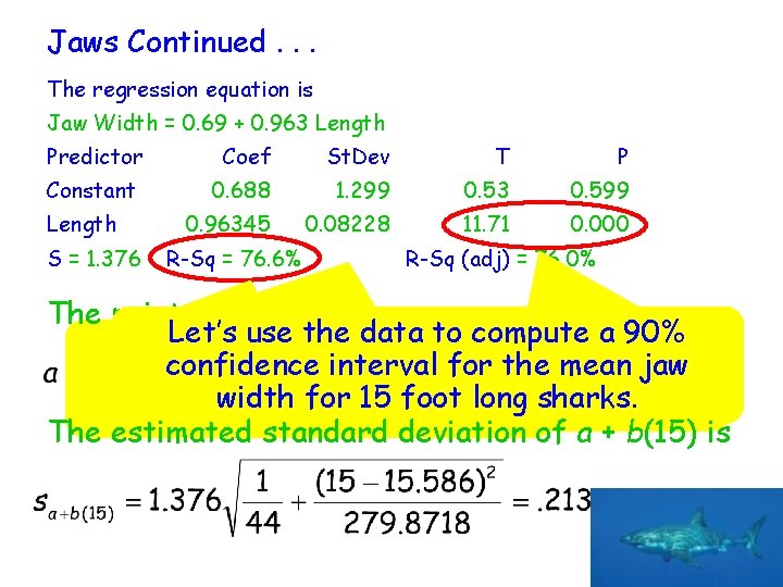
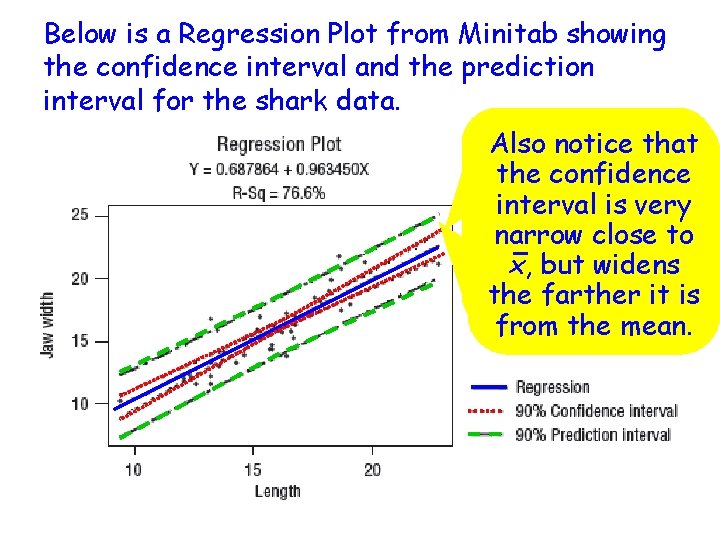
Physical characteristics of sharks are of interest to surfers and scuba divers as well as to marine researcher. The data on x = length (in feet) and y = jaw width (in inches) for 44 sharks (were found in various articles appearing in the magazines Skin Diver and Scuba News. (These data are found on page 778 of the text. ) Because it is difficult to measure jaw width in living sharks, researchers would like to determine whether it is possible to estimate jaw This widthscatterplot from body length, which is of the more easily measured. data shows a linear pattern and is consistent with use of the simple linear regression model.

Jaws Continued. . . The regression equation is Jaw Width = 0. 69 + 0. 963 Length Predictor Coef St. Dev T P Constant 0. 688 1. 299 0. 53 0. 599 0. 96345 0. 08228 11. 71 0. 000 Length S = 1. 376 R-Sq = 76. 6% R-Sq (adj) = 76. 0% The point estimate is use the data to compute a 90% The model utility test confirms The Let’s simple linear regression confidence interval thethis mean jaw the 76. 6% usefulness model explains offor theof width in for 15 width. foot long sharks. variability jaw The estimated standard deviation of a + b(15) is

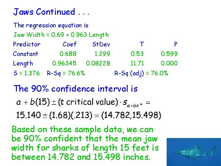
Jaws Continued. . . The regression equation is Jaw Width = 0. 69 + 0. 963 Length Predictor Coef St. Dev T P Constant 0. 688 1. 299 0. 53 0. 599 0. 96345 0. 08228 11. 71 0. 000 Length S = 1. 376 R-Sq = 76. 6% R-Sq (adj) = 76. 0% The 90% confidence interval is Based on these sample data, we can be 90% confident that the mean jaw width for sharks of length 15 feet is between 14. 782 and 15. 498 inches.

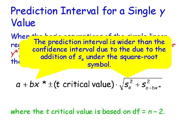
Prediction Interval for a Single y Value When the basic assumptions of the simple linear The model prediction interval is wider than thefor regression are met, a prediction interval The prediction interval and the confidence interval due to the y*, a confidence single y observation made when xat = x*, has interval are centered addition of se under the square-root exactly the samesymbol. place, a + bx*. the form where the t critical value is based on df = n – 2.

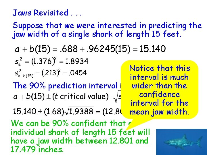
Jaws Revisited. . . Suppose that we were interested in predicting the jaw width of a single shark of length 15 feet. Notice that this interval is much The 90% prediction interval is wider than the confidence interval for the mean jaw width. We can be 90% confident that an individual shark of length 15 feet will have a jaw width between 12. 801 and 17. 479 inches.

Below is a Regression Plot from Minitab showing the confidence interval and the prediction interval for the shark data. Notice that the Also notice prediction the confidence interval is is very substantial narrow close to wider the x, butthan widens confidence the farther it is interval from the mean.

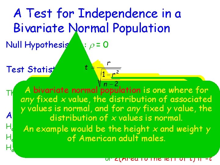
A Test for Independence in a Bivariate Normal Population Null Hypothesis: H 0: r = 0 Test Statistic: Greek letter “rho” coefficient. r is the population correlation Many investigators are However, r =interested 0 is NOT if ANY A relationship bivariate normal population is one where for assesses the extent of any linear The test is It based on df = n – 2. exist between y. That equivalent to x andx yand being any fixed value, the associated relationship in thedistribution population. rof must be is, arex x and y are independent of each independent except in the case y values is normal, and for y value, the between -1 any and fixed 1. other? of a bivariate Alternativedistribution Hypothesis: P-value: of xnormal values population. is normal. Ha: r An > 0 example (positive dependence) Area to thex right of t would be the height and weight y Ha: r < 0 (negativeof dependence) the left of t American. Area adulttomales. Ha: r ≠ 0 (dependence) 2(Area to the right of t) if +t or 2(Area to the left of t) if -t

A Test for Independence in a Bivariate Normal Population Assumptions: r is the correlation coefficient for a random sample from a bivariate normal population. The one way to verify that the population is a bivariate normal population is to plot individual normal probability plots of the x and y variables.

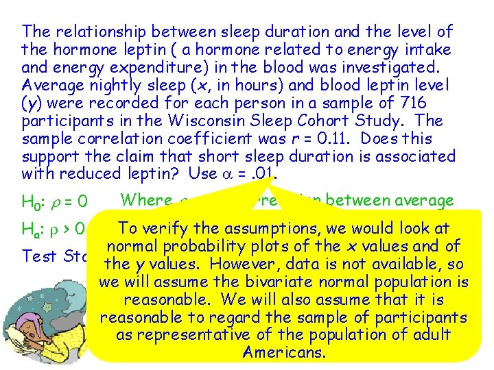
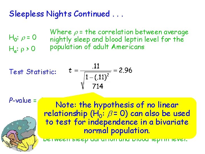
The relationship between sleep duration and the level of the hormone leptin ( a hormone related to energy intake and energy expenditure) in the blood was investigated. Average nightly sleep (x, in hours) and blood leptin level (y) were recorded for each person in a sample of 716 participants in the Wisconsin Sleep Cohort Study. The sample correlation coefficient was r = 0. 11. Does this support the claim that short sleep duration is associated with reduced leptin? Use a =. 01. Where r = the correlation between average nightly sleep and blood leptin level for the State the hypotheses. To verify the assumptions, we would look at Ha : r > 0 population of adult Americans normal probability plots of the x values and of Test Statistic: the y values. However, data is not available, so H 0 : r = 0 we will assume the bivariate normal population is reasonable. We will also assume that it is reasonable to regard the sample of participants as representative ofdfthe population ofaadult P-value =. 0015 = 714 =. 01 Americans.

Sleepless Nights Continued. . . H 0 : r = 0 Ha : r > 0 Where r = the correlation between average nightly sleep and blood leptin level for the population of adult Americans Test Statistic: P-value =. 0015 df = 714 a =. 01 Note: the hypothesis of no linear relationship (H 0<: . 01, b =we 0)reject can also used Since the P-value H 0. be There is to test to for independence evidence suggest that thereinisaa bivariate positive normal apopulation. association (perhaps weak one since r =. 11) between sleep duration and blood leptin level.