Chapter 13 Simple Linear Regression and Correlation Inferential

Chapter 13 Simple Linear Regression and Correlation: Inferential Methods

Objectives: •

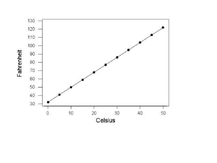
Suppose we were to investigate the relationship between y = the first-year college grade point average and x = high school grade point average. Is the first-year college grade point average determined solely by the high school grade point average? A relationship in which the value of y is completely determined by the value of an independent variable x is called a deterministic relationship.

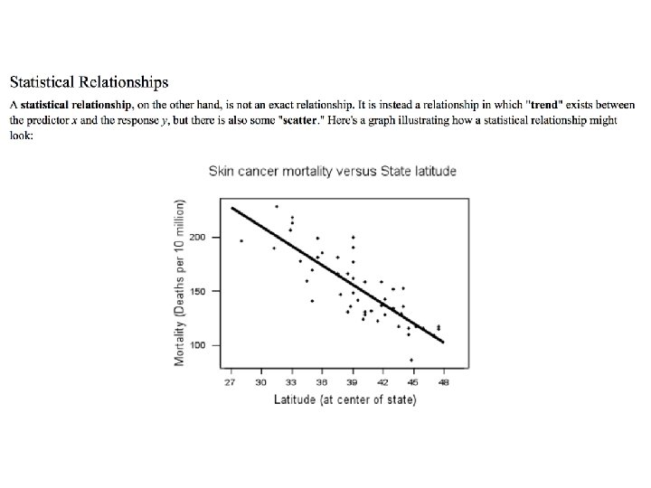
The first-year college grade point average and the high school grade point average do NOT have a deterministic relationship, rather Statistical relationship.

Examples of Statistical relationship (not exact relationship) • Height Vs. Weight • Driving speed Vs. gas mileage

The equation for an additive probabilistic model is: Where e is an “error” variable A description of the relationship between two variables that are not deterministically related can be given by a probabilistic model.

The simple linear regression model assumes that there is a line with y-intercept a and slope b, called the population regression line. When a value of the independent variable x is fixed an observation on the dependent variable y is made, y a Population regression line (slope b) e 1 Without the random deviation e in the 2 equation, all observed e(x, y) points would fall exactly on the population regression line. x 1 x 2 x

Assumptions of the Simple Linear Regression Model 1. The distribution of e at any particular x value has mean value 0. that is, me = 0. 2. The standard deviation of e is the same for any particular value of x. This standard deviation is denoted by s. 3. The distribution of e at any particular value of x is normal. 4. The random deviations e 1, e 2, . . . , en associated with different observations are independent of one another.

Let’s look at the heights and weights of a population of adult women. Weight How much Weights of women that Are some of these would an adult are 5 feet tall will vary We want the weights more likely Where would female weigh if What would – in other words, there standard This distribution is than others? you expect the is a distribution of she were 5 feet you expect deviations of all normally distributed. What would this population weights for adult tall? for other these normal distribution look females who are 5 feet regression line heights? tall. distributions to be like? to be? the same. Height

Interpretation of Terms 1. The slope of the population regression line is the mean (average) change in y associated with a 1 -unit increase in x. 3. The size of determines the extent to which the (x, y) observations deviate from the population line. Small s Large s

Estimates for the Regression Line We use to to estimate the true population regression line. b = point estimate of b, where a = point estimate of a, where, Note that b can also given by

Let x* denote a specific value of the predictor variable x. Then y=a + bx* has two different interpretations: 1. It is a point estimate of the mean y value when x = x*. 2. It is a point prediction of an individual y value to be observed when x = x*.

Example-Medical researches have noted that adolescent females are much more likely to deliver low-birth-weight babies than are adult females. Because low-birth-weight babies have higher mortality rates, a number of studies have examined the relationship between birth weight and mother’s age for babies born to young mothers. The following data is on x = maternal age (in years) and y = birth weight of baby (in grams). 15 17 18 15 17 16 18 19 The scatterplot shows a y 2289 3393 3271 2648 2897 3327 2535 3138 spread 3573 linear 2970 pattern and the in the y values appears to be similar across the range of x values. This supports the Sketch a scatterplot of these data. appropriateness of the simple linear regression model. Baby’s Weight (g) x Mother’s Age (yrs) 16 19

x 15 17 18 15 16 19 17 16 18 19 y 2289 3393 3271 2648 2897 3327 2970 2535 3138 3573 We can obtain the LSRL from GDC The estimated regression line is: y = -1163. 45 + 245. 15 x

The. Continued weight of. babies increase approximately 245. 15 grams Birth Weight. . for each increase of 1 year in the mother’s age. The following data is on x = maternal age (in years) and y = birth weight of baby (in grams). x 15 17 18 15 16 19 17 16 18 19 y 2289 3393 3271 2648 2897 3327 2970 2535 3138 3573 What is the point estimate for the mean weight of babies born to 18 -year-old mothers? Baby’s Weight (g) This is also the prediction of the weight of a single baby born to a This is the point estimate mother 18 years of age. for the mean weight of all babies born to 18 -year-old mothers. Mother’s Age (yrs)

Recall: Terminologies

The total sum of squares, denoted by SSTo, is defined as The residual sum of squares, denoted by SSResid, is defined as

SSTo and SSResid are generally found as part of the standard output from most statistical packages or can be obtained using the following computational formulas:

Coefficient of Determination • The coefficient of determination, denoted by r 2, gives the proportion of variation in y that can be attributed to an approximate linear relationship between x and y.

The statistic for estimating the variance s 2 is where Why n – 2? The estimate for the standard deviation s is Since we must estimate both for a Note that the degrees of freedom The subscript e reminds us that and b in the regression line, we associated with estimating s 2 or s in we are estimating the variance reduce the sample size n by 2 simple linear regression is of the “errors” or residuals. df = n - 2

3 Questions to be done in pairs!

Wednesday/Monday? • Test on Ch-12 + 13