Ch 11 Introduction to RNN LSTM RNN Recurrent

Ch. 11 : Introduction to RNN, LSTM RNN (Recurrent neural network) LSTM (Long short-term memory) KH Wong Ch 11. RNN, LSTM v. 1 c (21 -22) 1

Overview • • • Introduction Concept of RNN (Recurrent neural network) ? The Gradient vanishing problem LSTM theory and concept LSTM Numerical example Ch 11. RNN, LSTM v. 1 c (21 -22) 2

Introduction • RNN (Recurrent neural network) is a form of neural networks that feed outputs back to the inputs during operation • LSTM (Long short-term memory) is a form of RNN. It fixes the vanishing gradient problem of the original RNN. – Application: Sequence to sequence model based using LSTM for machine translation • • • References: Materials are mainly based on links found in https: //www. tensorflow. org/tutorials https: //towardsdatascience. com/illustrated-guide-to-lstms-and-gru-s-a-step-by-step-explanation 44 e 9 eb 85 bf 21 Ch 11. RNN, LSTM v. 1 c (21 -22) 3

Concept of RNN (Recurrent neural network) concept Ch 11. RNN, LSTM v. 1 c (21 -22) 4

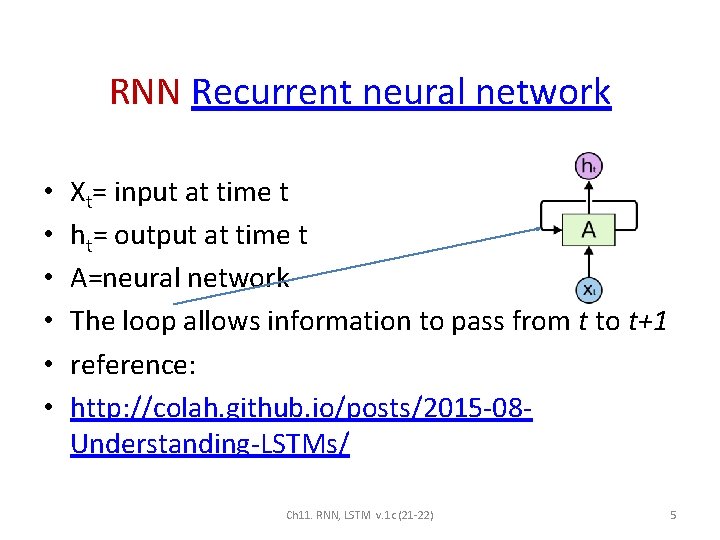
RNN Recurrent neural network • • • Xt= input at time t ht= output at time t A=neural network The loop allows information to pass from t to t+1 reference: http: //colah. github. io/posts/2015 -08 Understanding-LSTMs/ Ch 11. RNN, LSTM v. 1 c (21 -22) 5

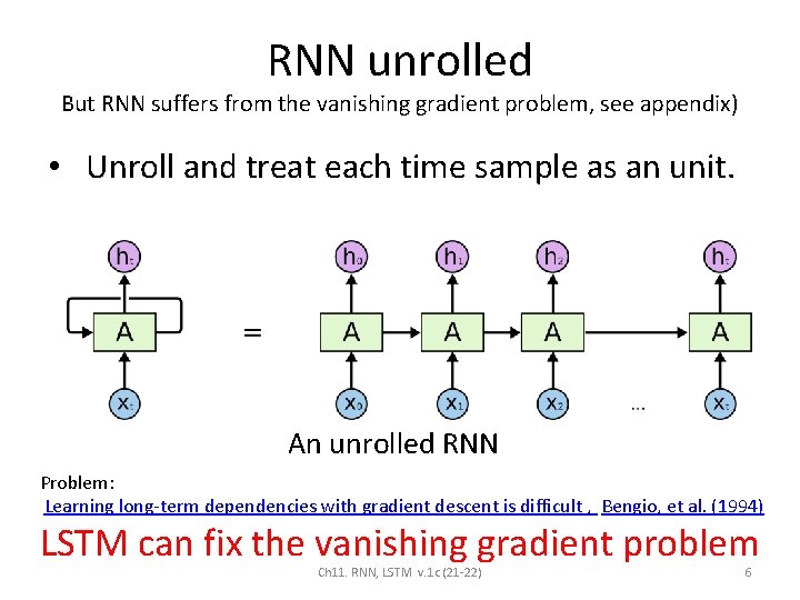
RNN unrolled But RNN suffers from the vanishing gradient problem, see appendix) • Unroll and treat each time sample as an unit. An unrolled RNN Problem: Learning long-term dependencies with gradient descent is difficult , Bengio, et al. (1994) LSTM can fix the vanishing gradient problem Ch 11. RNN, LSTM v. 1 c (21 -22) 6

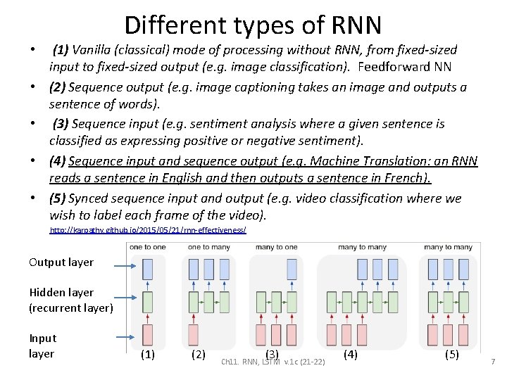
• • • Different types of RNN (1) Vanilla (classical) mode of processing without RNN, from fixed-sized input to fixed-sized output (e. g. image classification). Feedforward NN (2) Sequence output (e. g. image captioning takes an image and outputs a sentence of words). (3) Sequence input (e. g. sentiment analysis where a given sentence is classified as expressing positive or negative sentiment). (4) Sequence input and sequence output (e. g. Machine Translation: an RNN reads a sentence in English and then outputs a sentence in French). (5) Synced sequence input and output (e. g. video classification where we wish to label each frame of the video). http: //karpathy. github. io/2015/05/21/rnn-effectiveness/ Output layer Hidden layer (recurrent layer) Input layer (1) (2) (3) Ch 11. RNN, LSTM v. 1 c (21 -22) (4) (5) 7

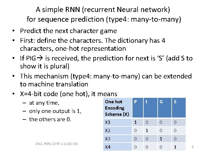
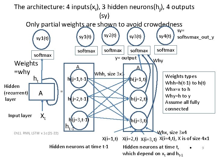
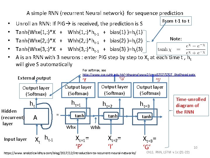
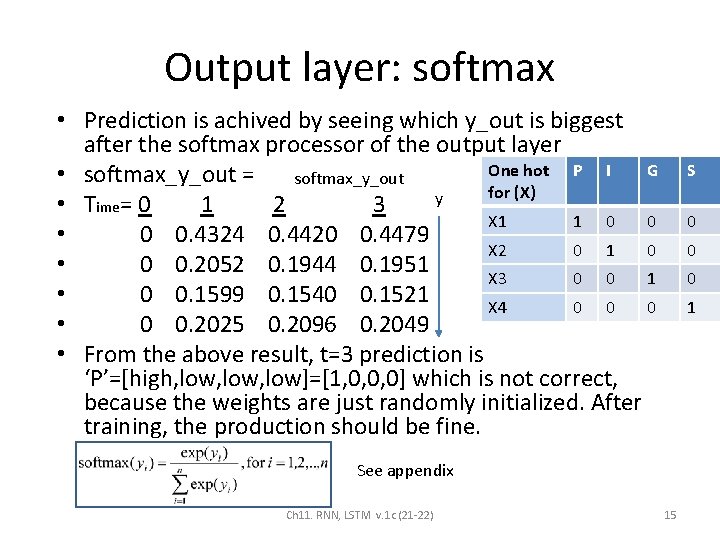
A simple RNN (recurrent Neural network) for sequence prediction (type 4: many-to-many) • Predict the next character game • First: define the characters. The dictionary has 4 characters, one-hot representation • If PIG is received, the prediction for next is ‘S’ (add S to show it is plural) • This mechanism (type 4: many-to-many) can be extended to machine translation • X=4 -bit code (one hot), it means – at any time, – only one output is 1, – the others are 0. Ch 11. RNN, LSTM v. 1 c (21 -22) One hot Encoding Scheme (X) P I G S X 1 1 0 0 0 X 2 0 1 0 0 X 3 0 0 1 0 X 4 0 0 0 1 8

The architecture: 4 inputs(xi), 3 hidden neurons(hj), 4 outputs (sy) Only partial weights are shown to avoid crowdedness softmax Weights =why ht Hidden (recurrent) layer Input layer sy 2(t) sy 1(t) softmax y= output A h(j=1, t-1) sy 3(t) Whh, size 3 x 3 Xt h(j=1, t) h(j=2, t-1) h(j=2, t) h(j=3, t-1) h(j=3, t) ht-1 softmax Why A = A sy 4(t) sy= softwmax_out_y Weights types Whh=h(t-1) to h(t) Whx=x to h Why=h to y Assume all fully connected Whx, size 3 x 4 X(i=1, t) X(i=2, t) X(i=3, t) X(i=4, t), X is of size 4 x 1 Hidden neurons at time t-1 Hidden neurons at time t, 9 • which depend on xt and ht-1 Ch 11. RNN, LSTM v. 1 c (21 -22)

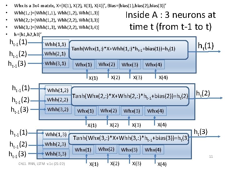
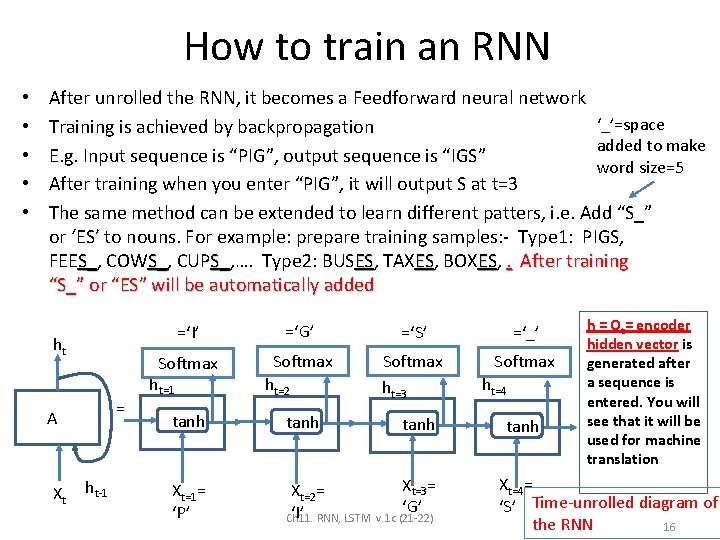
A simple RNN (recurrent Neural network) for sequence prediction • • • From t-1 to t Unroll an RNN: If PIG is received, the prediction is S Tanh(Whx(1, : )*X + Whh(1, : )*ht-1 + bias(1) )=ht(1) Note: Tanh(Whx(2, : )*X + Whh(2, : )*ht-1 + bias(2) )=ht(2) Tanh(Whx(3, : )*X + Whh(3, : )*ht-1 + bias(3) )=ht(3) A is an RNN with 3 neurons : enter PIG step by step to Xt at each time t , ht will give S automatically For softmax, see http: //www. cse. cuhk. edu. hk/~khwong/www 2/cmsc 5707/5707_likelihood. pptx External output ‘I’ Output layer (Softmax) Hidden (recurrent) layer Input layer ht=1 ht A = Xt ht-1 Xt=1= ‘P’ Output layer (Softmax) ht=2 tanh Whx ‘G’ ‘S’ Output layer (Softmax) ht=3 tanh Xt=2= ‘I’ Xt=3= ‘G’ Time-unrolled diagram of the RNN Whh https: //www. analyticsvidhya. com/blog/2017/12/introduction-to-recurrent-neural-networks/ Ch 11. RNN, LSTM v. 1 c (21 -22) 10

• • • Whx is a 3 x 4 matrix, X=[X(1), X(2), X(3), X(4)]’, Bias=[bias(1), bias(2), bias(3)]’ Whh(1, : )=[Whh(1, 1), Whh(1, 2), Whh(1, 3)] Whh(2, : )=[Whh(1, 2), Whh(2, 2), Whh(3, 3)] Whh(3, : )=[Whh(1, 3), Whh(2, 2), Whh(3, 4)] h=[h 1, h 2, h 3]’ Inside A : 3 neurons at time t (from t-1 to t) ht-1(1) ht-1(2) ht-1(3) Whh(1, 1) Whh(2, 1) Whh(3, 1) Tanh(Whx(1, : )*X+Whh(1, : )*ht-1+bias(1))=ht(1) Whx(2) Whx(1) X(1) ht-1(2) ht-1(3) ht-1(1) ht-1(2) ht-1(3) Whh(1, 2) Whh(2, 2) Whh(3, 2) Whh(2, 3) Whh(3, 3) Ch 11. RNN, LSTM v. 1 c (21 -22) X(3) Whx(4) X(4) Tanh(Whx(2, : )*X+Whh(2, : )*ht-1+bias(2))=ht(2) Whx(1) X(2) X(1) Whh(1, 3) X(2) Whx(3) X(3) Whx(2) Whx(3) ht(2) Whx(4) X(4) Tanh(Whx(3, : )*X+Whh(3, : )*ht-1+bias(3))=ht(3) Whx(1) ht(3) Whx(4) 11 X(1) X(2) X(3) X(4)

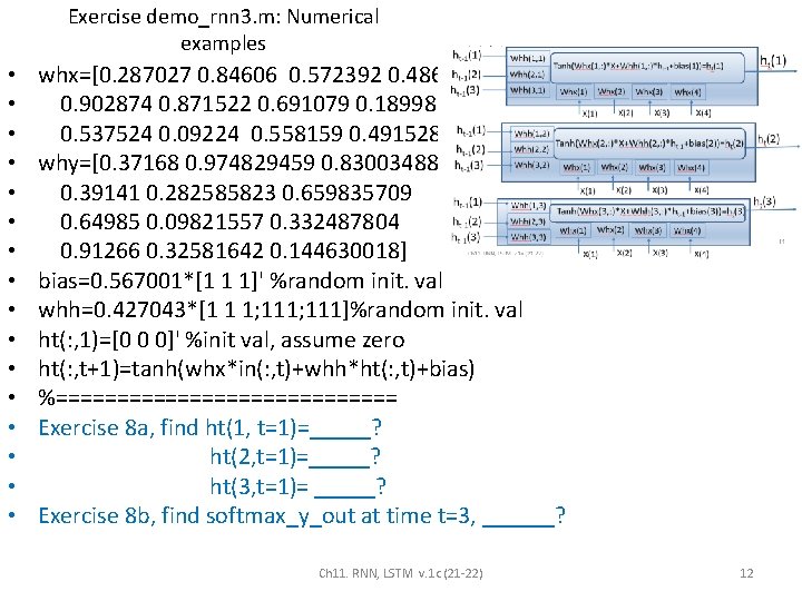
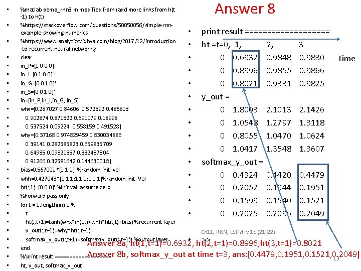
Exercise demo_rnn 3. m: Numerical examples • • • • whx=[0. 287027 0. 84606 0. 572392 0. 486813 0. 902874 0. 871522 0. 691079 0. 18998 0. 537524 0. 09224 0. 558159 0. 491528] why=[0. 37168 0. 974829459 0. 830034886 0. 39141 0. 282585823 0. 659835709 0. 64985 0. 09821557 0. 332487804 0. 91266 0. 32581642 0. 144630018] bias=0. 567001*[1 1 1]' %random init. val whh=0. 427043*[1 1 1; 111]%random init. val ht(: , 1)=[0 0 0]' %init val, assume zero ht(: , t+1)=tanh(whx*in(: , t)+whh*ht(: , t)+bias) %============== Exercise 8 a, find ht(1, t=1)=_____? ht(2, t=1)=_____? ht(3, t=1)= _____? Exercise 8 b, find softmax_y_out at time t=3, ______? Ch 11. RNN, LSTM v. 1 c (21 -22) 12

• • • • • • • Answer 8 %matlab demo_rnn 3. m modified from (add more links from h(t -1) to h(t) %https: //stackoverflow. com/questions/50050056/simple-rnn • print result ========== example-showing-numerics %https: //www. analyticsvidhya. com/blog/2017/12/introduction • ht =t=0, 1, 2, 3 -to-recurrent-neural-networks/ clear • 0 0. 6932 0. 9848 0. 9830 Time in_P=[1 0 0 0]' • 0 0. 8996 0. 9855 0. 9866 in_I=[0 1 0 0]' in_G=[0 0 1 0]' • 0 0. 8021 0. 9331 0. 9825 in_S=[0 0 1 0]' • y_out = in=[in_P, in_I, in_G, in_S] whx=[0. 287027 0. 84606 0. 572392 0. 486813 • 0 1. 8003 2. 1013 2. 1426 0. 902874 0. 871522 0. 691079 0. 18998 • 0 1. 0548 1. 2797 1. 3118 0. 537524 0. 09224 0. 558159 0. 491528] why=[0. 37168 0. 974829459 0. 830034886 • 0 0. 8055 1. 0470 1. 0624 0. 39141 0. 282585823 0. 659835709 • 0 1. 0417 1. 3548 1. 3607 0. 64985 0. 09821557 0. 332487804 0. 91266 0. 32581642 0. 144630018] • softmax_y_out = bias=0. 567001*[1 1 1]' %random init. val • 0 0. 4324 0. 4420 0. 4479 whh=0. 427043*[1 1 1; 1 1 1]%random init. Val ht(: , 1)=[0 0 0]' %init val, assume zero • 0 0. 2052 0. 1944 0. 1951 %Forward pass only • 0 0. 1599 0. 1540 0. 1521 for t = 1: length(in)-1 % t • 0 0. 2025 0. 2096 0. 2049 ht(: , t+1)=tanh(whx*in(: , t)+whh*ht(: , t)+bias) %recurrent layer y_out(: , t+1)=why*ht(: , t+1) Ch 11. RNN, LSTM v. 1 c (21 -22) softmax_y_out(: , t+1)=softmax(y_out(: , t+1)) %output layer • ht(2, t=1)=0. 8996, ht(3, t=1)=0. 8021 >> Answer 8 a, ht(1, t=1)=0. 6932, end Answer 8 b, softmax_y_out at time t=3, ans: [0. 4479, 0. 1951, 0. 1521, 0. 2049] %'print result ==========‘ 13 ht, y_out, softmax_y_out

Answer RNN 1 b • • • • Softmax is to make sum_all_i{softmax[y_out(i)]}=1 , each softmax[y_out(i)] is a probability print result ========== ht , t=0, 1, 2, 3 0 0. 6932 0. 9848 0. 9830 0 0. 8996 0. 9855 0. 9866 0 0. 8021 0. 9331 0. 9825 y_out = 0 1. 8003 2. 1013 2. 1426 0 1. 0548 1. 2797 1. 3118 The 0 0. 8055 1. 0470 1. 0624 output 0 1. 0417 1. 3548 1. 3607 layer softmax_y_out = 0 0. 4324 0. 4420 0. 4479 0 0. 2052 0. 1944 0. 1951 0 0. 1599 0. 1540 0. 1521 0 0. 2025 0. 2096 0. 2049 Time 0 1 2 3 Softmax[y_outi] i=1, 2, 3, 4 Y_outi=1, 2, 3, 4 Weights: Why (4 x 3) ht(1) ht(2) ht(3) Ch 11. RNN, LSTM v. 1 c (21 -22) 14

Output layer: softmax • Prediction is achived by seeing which y_out is biggest after the softmax processor of the output layer One hot P I G • softmax_y_out = softmax_y_out for (X) y • Time= 0 1 2 3 X 1 1 0 0 • 0 0. 4324 0. 4420 0. 4479 X 2 0 1 0 • 0 0. 2052 0. 1944 0. 1951 X 3 0 0 1 • 0 0. 1599 0. 1540 0. 1521 X 4 0 0 0 • 0 0. 2025 0. 2096 0. 2049 • From the above result, t=3 prediction is ‘P’=[high, low, low]=[1, 0, 0, 0] which is not correct, because the weights are just randomly initialized. After training, the production should be fine. S 0 0 0 1 See appendix Ch 11. RNN, LSTM v. 1 c (21 -22) 15

How to train an RNN • • • After unrolled the RNN, it becomes a Feedforward neural network ‘_’=space Training is achieved by backpropagation added to make E. g. Input sequence is “PIG”, output sequence is “IGS” word size=5 After training when you enter “PIG”, it will output S at t=3 The same method can be extended to learn different patters, i. e. Add “S_” or ‘ES’ to nouns. For example: prepare training samples: - Type 1: PIGS, FEES_, Type 2: BUSES, S_ COWS_, S_ CUPS_, …. S_ ES TAXES, ES BOXES, ES. After training “S_” or “ES” will be automatically added ht = A Xt ht-1 =‘I’ =‘G’ =‘S’ =‘_’ Softmax ht=1 Softmax ht=2 Softmax ht=3 Softmax tanh Xt=1= ‘P’ Xt=2= ‘I’ RNN, LSTM Ch 11. Xt=3= ‘G’ v. 1 c (21 -22) ht=4 tanh h = Ot= encoder hidden vector is generated after a sequence is entered. You will see that it will be used for machine translation Xt=4= ‘S’ Time-unrolled diagram of the RNN 16

Problem with RNN: The vanishing gradient problem Ref: https: //hackernoon. com/exploding-and-vanishing-gradient-problem-math-behind-the-truth 6 bd 008 df 6 e 25 Ch 11. RNN, LSTM v. 1 c (21 -22) 17

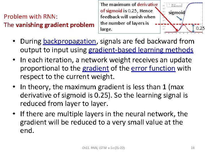
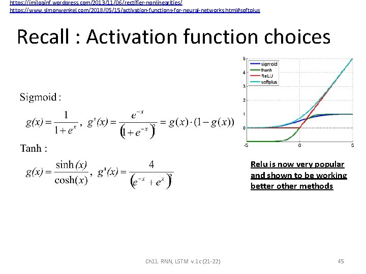
Problem with RNN: The vanishing gradient problem The maximum of derivative of sigmoid is 0. 25, Hence feedback will vanish when the number of layers is large. sigmoid 0. 25 • During backpropagation, signals are fed backward from output to input using gradient-based learning methods • In each iteration, a network weight receives an update proportional to the gradient of the error function with respect to the current weight. • In theory, the maximum gradient is less than 1 (max derivative of sigmoid is 0. 25). So the learning signal is reduced from layer to layer. • If there are multiple layers in the neural network, the gradient will be reduced to a very small value at the end. Ch 11. RNN, LSTM v. 1 c (21 -22) 18

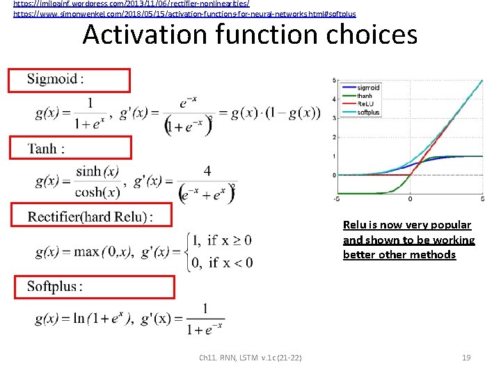
https: //imiloainf. wordpress. com/2013/11/06/rectifier-nonlinearities/ https: //www. simonwenkel. com/2018/05/15/activation-functions-for-neural-networks. html#softplus Activation function choices Relu is now very popular and shown to be working better other methods Ch 11. RNN, LSTM v. 1 c (21 -22) 19

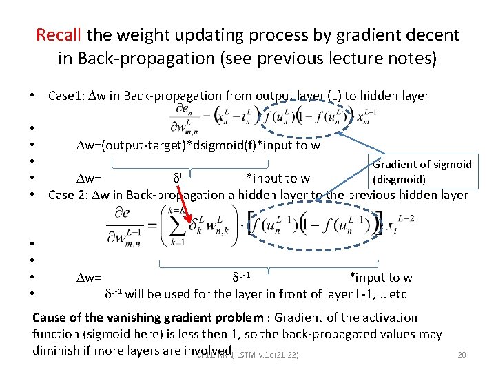
Recall the weight updating process by gradient decent in Back-propagation (see previous lecture notes) • Case 1: w in Back-propagation from output layer (L) to hidden layer • • w=(output-target)*dsigmoid(f)*input to w • Gradient of sigmoid L • w= *input to w (disgmoid) • Case 2: w in Back-propagation a hidden layer to the previous hidden layer • • w= L-1 *input to w L-1 will be used for the layer in front of layer L-1, . . etc Cause of the vanishing gradient problem : Gradient of the activation function (sigmoid here) is less then 1, so the back-propagated values may diminish if more layers are involved Ch 11. RNN, LSTM v. 1 c (21 -22) 20

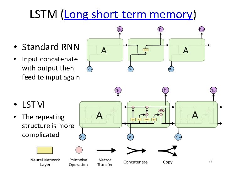
To solve the vanishing gradient problem, LSTM adds C (cell state) • RNN has xi (input) and ht (output) only • In LSTM, add – Cell state (Ct) to solve gradient vanishing problem – In each time (t), updates • Ct=cell state (ranges from -1 to 1) • ht= output (ranges from 0 to 1) • The system learns Ct and ht together Ch 11. RNN, LSTM v. 1 c (21 -22) 21

LSTM (Long short-term memory) • Standard RNN • Input concatenate with output then feed to input again • LSTM • The repeating structure is more complicated Ch 11. RNN, LSTM v. 1 c (21 -22) 22

Stacked LSTM Stacked Long short-term memory Hierarchical structure Theory and concept Ch 11. RNN, LSTM v. 1 c (21 -22) 23

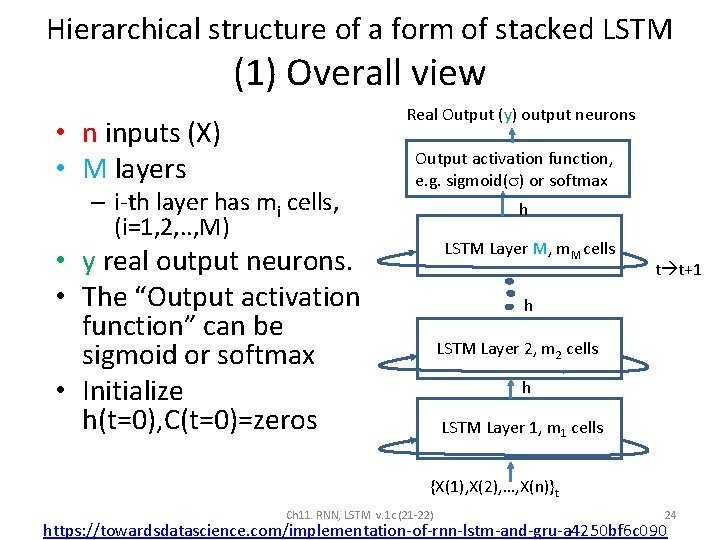
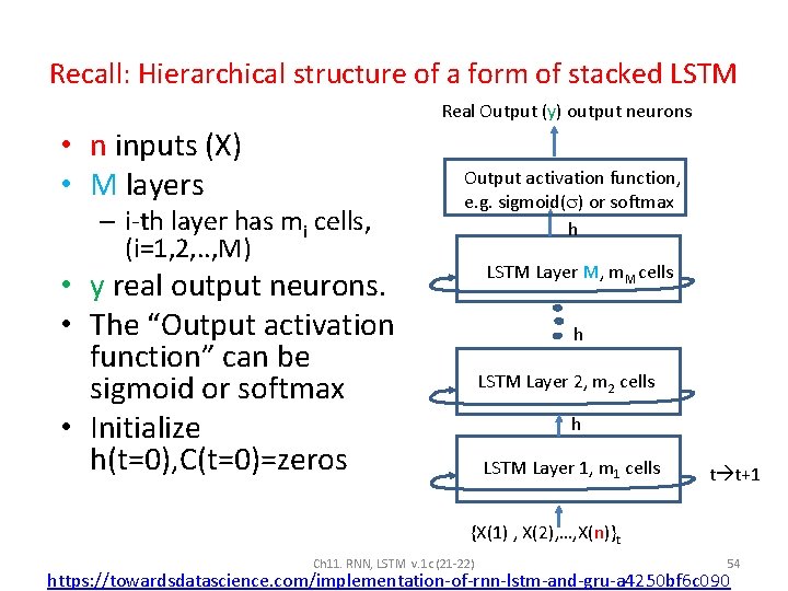
Hierarchical structure of a form of stacked LSTM (1) Overall view Real Output (y) output neurons • n inputs (X) • M layers – i-th layer has mi cells, (i=1, 2, . . , M) Output activation function, e. g. sigmoid( ) or softmax h LSTM Layer M, m. M cells • y real output neurons. • The “Output activation function” can be sigmoid or softmax • Initialize h(t=0), C(t=0)=zeros t t+1 h LSTM Layer 2, m 2 cells h LSTM Layer h 1, m 1 cells {X(1), X(2), …, X(n)}t Ch 11. RNN, LSTM v. 1 c (21 -22) 24 https: //towardsdatascience. com/implementation-of-rnn-lstm-and-gru-a 4250 bf 6 c 090

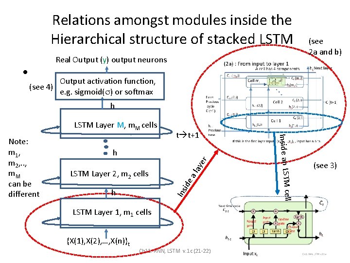
Relations amongst modules inside the Hierarchical structure of stacked LSTM Real Output (y) output neurons • (see 4) (see 2 a and b) Output activation function, e. g. sigmoid( ) or softmax h LSTM Layer M, m. M cells al (see 3) cell h Ins ide LSTM Layer 2, m 2 cells ay er h Inside an LSTM Note: m 1, m 2, . . , m. M can be different t t+1 LSTM Layer h 1, m 1 cells {X(1), X(2), …, X(n)}t Ch 11. RNN, LSTM v. 1 c (21 -22) 25

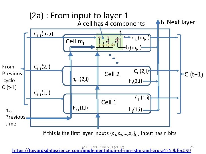
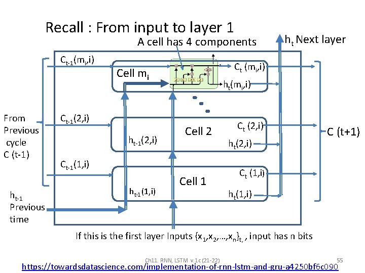
(2 a) : From input to layer 1 A cell has 4 components Ct-1(mi, i) From Previous cycle C (t-1) ht-1 Previous time Ct (mi, i) Cell mi Ct-1(2, i) ht(mi, i) Cell 2 Ct-1(1, i) ht Next layer Cell 1 Ct (2, i) ht(2, i) C (t+1) Ct (1, i) ht(1, i) If this is the first layer Inputs {x 1, x 2, …, xn}t, , input has n bits Ch 11. RNN, LSTM v. 1 c (21 -22) 26 https: //towardsdatascience. com/implementation-of-rnn-lstm-and-gru-a 4250 bf 6 c 090

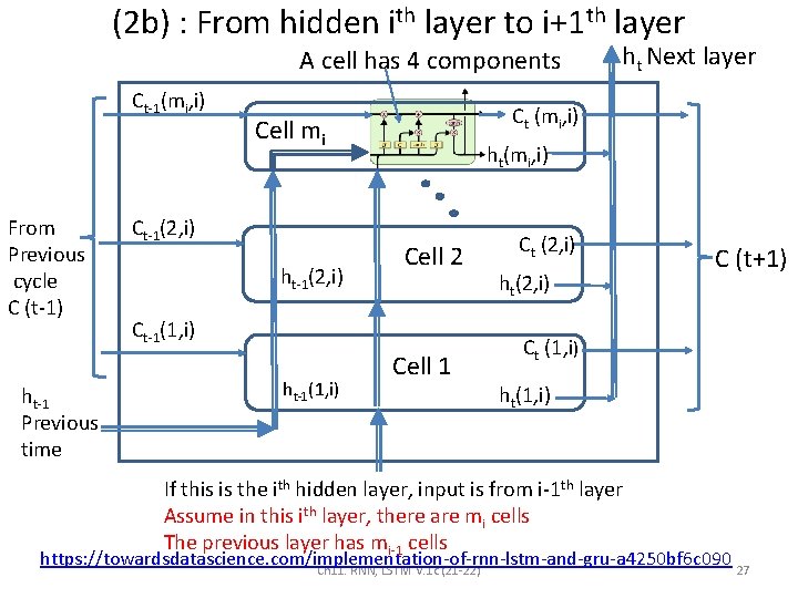
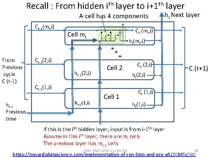
(2 b) : From hidden ith layer to i+1 th layer A cell has 4 components Ct-1(mi, i) From Previous cycle C (t-1) ht-1 Previous time Ct (mi, i) Cell mi Ct-1(2, i) ht(mi, i) Cell 2 Ct-1(1, i) ht Next layer Cell 1 Ct (2, i) ht(2, i) C (t+1) Ct (1, i) ht(1, i) If this is the ith hidden layer, input is from i-1 th layer Assume in this ith layer, there are mi cells The previous layer has mi-1 cells https: //towardsdatascience. com/implementation-of-rnn-lstm-and-gru-a 4250 bf 6 c 090 Ch 11. RNN, LSTM v. 1 c (21 -22) 27

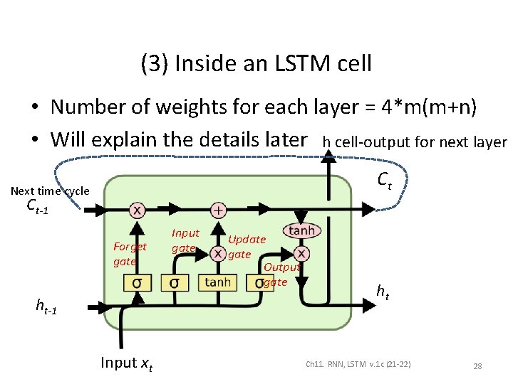
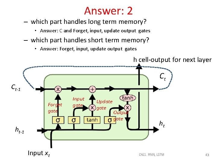
(3) Inside an LSTM cell • Number of weights for each layer = 4*m(m+n) • Will explain the details later h cell-output for next layer Ct Next time cycle Ct-1 Forget gate ht-1 Input xt Input gate Update gate Output gate ht Ch 11. RNN, LSTM v. 1 c (21 -22) 28

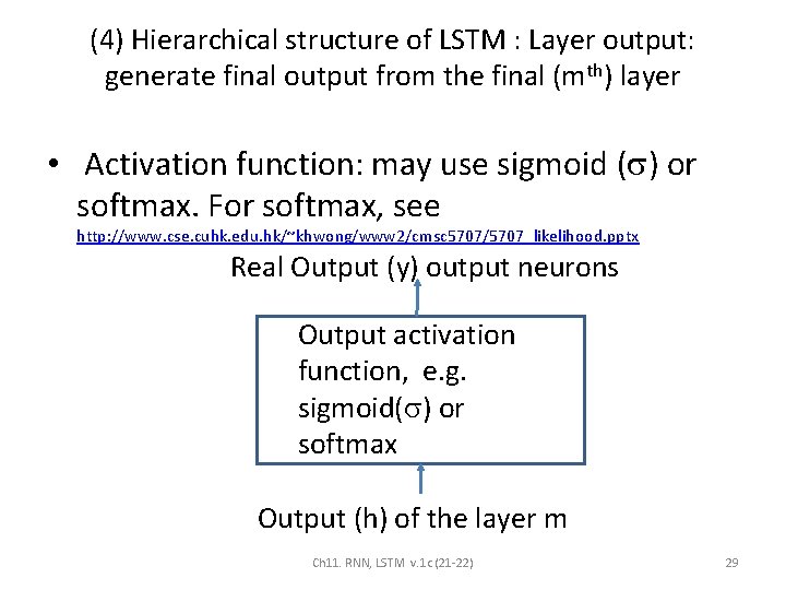
(4) Hierarchical structure of LSTM : Layer output: generate final output from the final (mth) layer • Activation function: may use sigmoid ( ) or softmax. For softmax, see http: //www. cse. cuhk. edu. hk/~khwong/www 2/cmsc 5707/5707_likelihood. pptx Real Output (y) output neurons Output activation function, e. g. sigmoid( ) or softmax Output (h) of the layer m Ch 11. RNN, LSTM v. 1 c (21 -22) 29

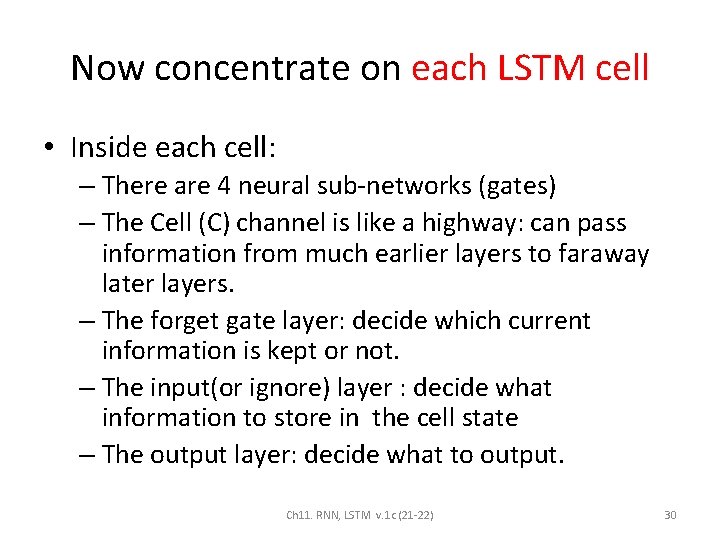
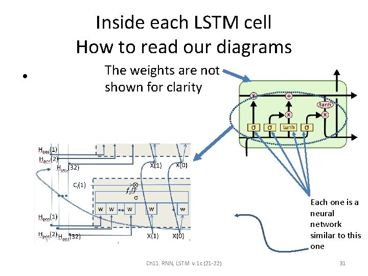
Now concentrate on each LSTM cell • Inside each cell: – There are 4 neural sub-networks (gates) – The Cell (C) channel is like a highway: can pass information from much earlier layers to faraway later layers. – The forget gate layer: decide which current information is kept or not. – The input(or ignore) layer : decide what information to store in the cell state – The output layer: decide what to output. Ch 11. RNN, LSTM v. 1 c (21 -22) 30

Inside each LSTM cell How to read our diagrams • The weights are not shown for clarity Each one is a neural network similar to this one Ch 11. RNN, LSTM v. 1 c (21 -22) 31

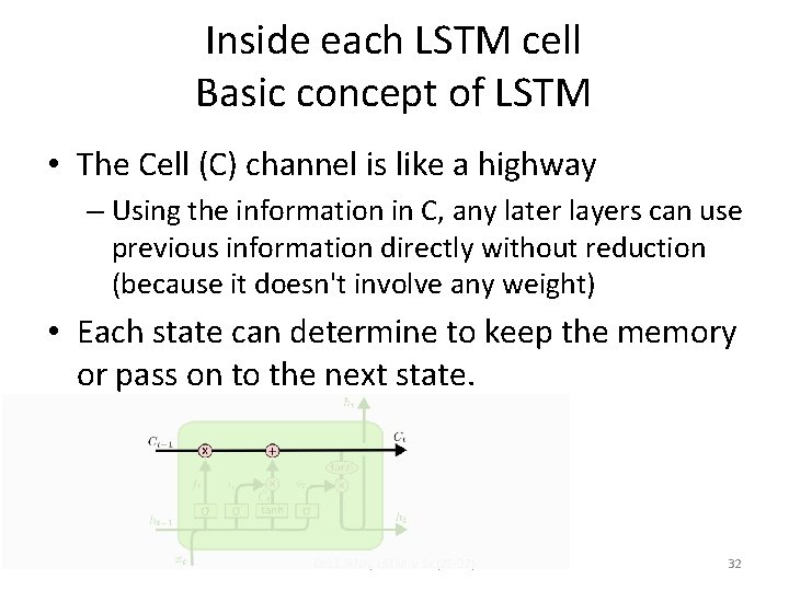
Inside each LSTM cell Basic concept of LSTM • The Cell (C) channel is like a highway – Using the information in C, any later layers can use previous information directly without reduction (because it doesn't involve any weight) • Each state can determine to keep the memory or pass on to the next state. Ch 11. RNN, LSTM v. 1 c (21 -22) 32

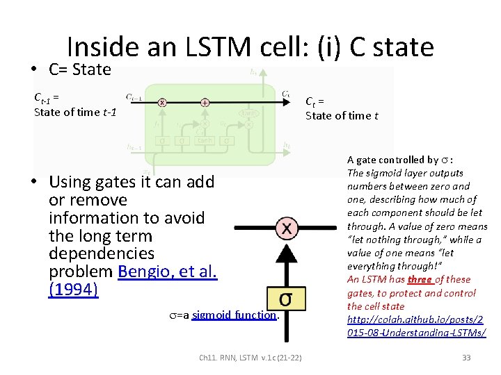
Inside an LSTM cell: (i) C state • C= State Ct-1 = State of time t-1 Ct = State of time t • Using gates it can add or remove information to avoid the long term dependencies problem Bengio, et al. (1994) =a sigmoid function. Ch 11. RNN, LSTM v. 1 c (21 -22) A gate controlled by : The sigmoid layer outputs numbers between zero and one, describing how much of each component should be let through. A value of zero means “let nothing through, ” while a value of one means “let everything through!” An LSTM has three of these gates, to protect and control the cell state http: //colah. github. io/posts/2 015 -08 -Understanding-LSTMs/ 33

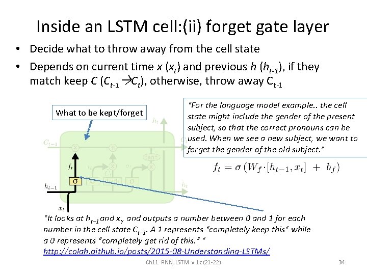
Inside an LSTM cell: (ii) forget gate layer • Decide what to throw away from the cell state • Depends on current time x (xt) and previous h (ht-1), if they match keep C (Ct-1 Ct), otherwise, throw away Ct-1 What to be kept/forget “For the language model example. . the cell state might include the gender of the present subject, so that the correct pronouns can be used. When we see a new subject, we want to forget the gender of the old subject. ” “It looks at ht− 1 and xt, and outputs a number between 0 and 1 for each number in the cell state Ct− 1. A 1 represents “completely keep this” while a 0 represents “completely get rid of this. ” ” http: //colah. github. io/posts/2015 -08 -Understanding-LSTMs/ Ch 11. RNN, LSTM v. 1 c (21 -22) 34

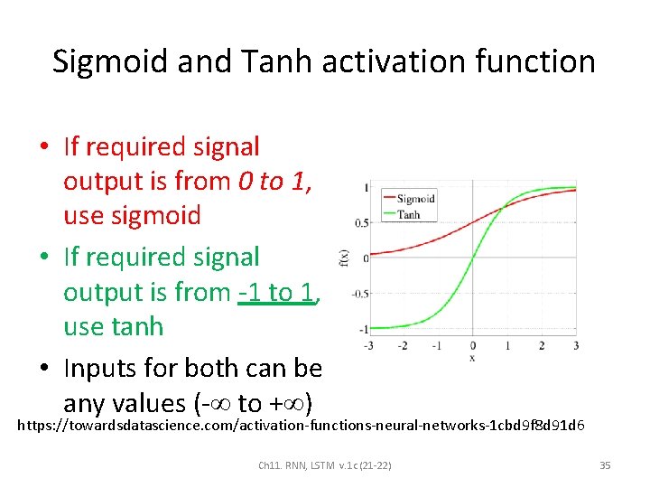
Sigmoid and Tanh activation function • If required signal output is from 0 to 1, use sigmoid • If required signal output is from -1 to 1, use tanh • Inputs for both can be any values (- to + ) https: //towardsdatascience. com/activation-functions-neural-networks-1 cbd 9 f 8 d 91 d 6 Ch 11. RNN, LSTM v. 1 c (21 -22) 35

Exercise 1 • What is the difference between Sigmoid and Tanh activation function? • Under what situation you will use Sigmoid activation function? • Under what situation you will use Tanh activation function? Ch 11. RNN, LSTM v. 1 c (21 -22) 36

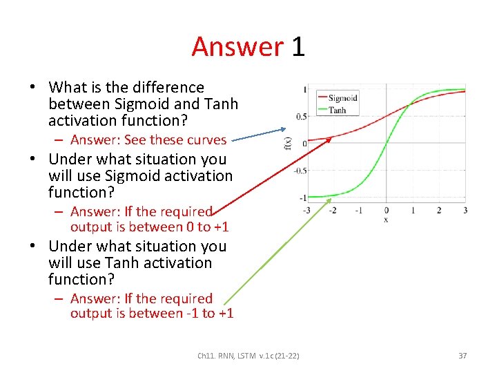
Answer 1 • What is the difference between Sigmoid and Tanh activation function? – Answer: See these curves • Under what situation you will use Sigmoid activation function? – Answer: If the required output is between 0 to +1 • Under what situation you will use Tanh activation function? – Answer: If the required output is between -1 to +1 Ch 11. RNN, LSTM v. 1 c (21 -22) 37

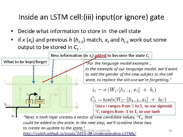
Inside an LSTM cell: (iii) input(or ignore) gate • Decide what information to store in the cell state • if x (xt) and previous h (ht-1) match, xt and ht-1 work out some output to be stored in Ct. What to be kept/forget New information (in xt) added to become the state Ct “For the language model example. . In the example of our language model, we’d want to add the gender of the new subject to the cell state, to replace the old one we’re forgetting. ” Since i ranges from 0 to 1, so use sigmoid; ~C ranges from -1 to 1, so use tanh t “Next, a tanh layer creates a vector of new candidate values, ~Ct, that could be added to the state. In the next step, we’ll combine these two to create an update to the Ch 11. state. ” RNN, LSTM v. 1 c (21 -22) 38 http: //colah. github. io/posts/2015 -08 -Understanding-LSTMs/

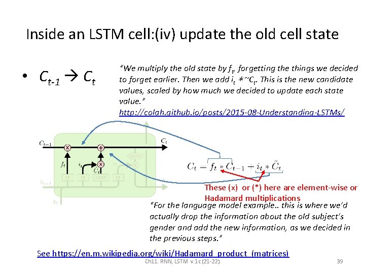
Inside an LSTM cell: (iv) update the old cell state • Ct-1 Ct “We multiply the old state by ft, forgetting the things we decided to forget earlier. Then we add it ∗ ~Ct. This is the new candidate values, scaled by how much we decided to update each state value. ” http: //colah. github. io/posts/2015 -08 -Understanding-LSTMs/ These (x) or (*) here are element-wise or Hadamard multiplications “For the language model example. . this is where we’d actually drop the information about the old subject’s gender and add the new information, as we decided in the previous steps. ” See https: //en. m. wikipedia. org/wiki/Hadamard_product_(matrices) Ch 11. RNN, LSTM v. 1 c (21 -22) 39

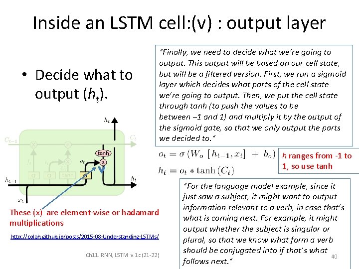
Inside an LSTM cell: (v) : output layer • Decide what to output (ht). “Finally, we need to decide what we’re going to output. This output will be based on our cell state, but will be a filtered version. First, we run a sigmoid layer which decides what parts of the cell state we’re going to output. Then, we put the cell state through tanh (to push the values to be between − 1 and 1) and multiply it by the output of the sigmoid gate, so that we only output the parts we decided to. ” h ranges from -1 to 1, so use tanh These (x) are element-wise or hadamard multiplications http: //colah. github. io/posts/2015 -08 -Understanding-LSTMs/ Ch 11. RNN, LSTM v. 1 c (21 -22) “For the language model example, since it just saw a subject, it might want to output information relevant to a verb, in case that’s what is coming next. For example, it might output whether the subject is singular or plural, so that we know what form a verb should be conjugated into if that’s what 40 follows next. ”

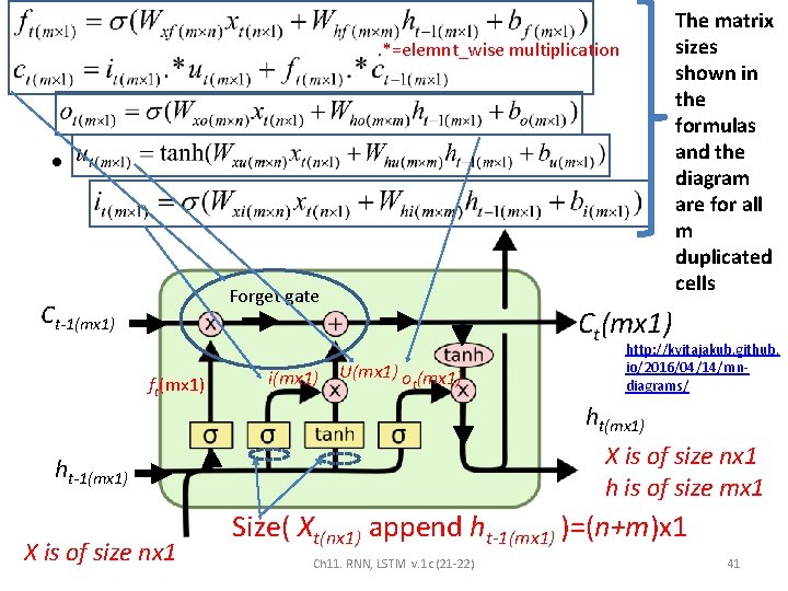
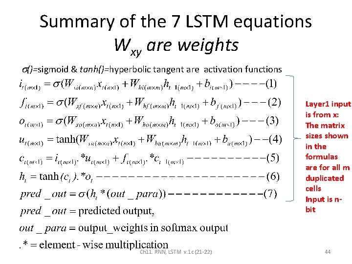
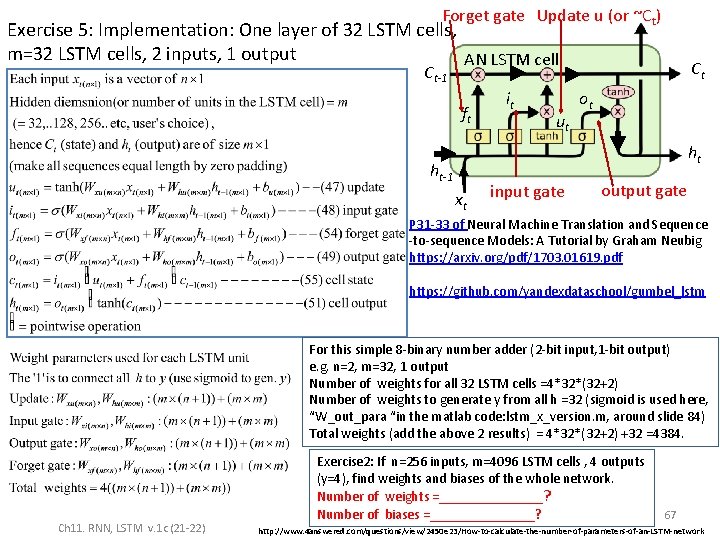
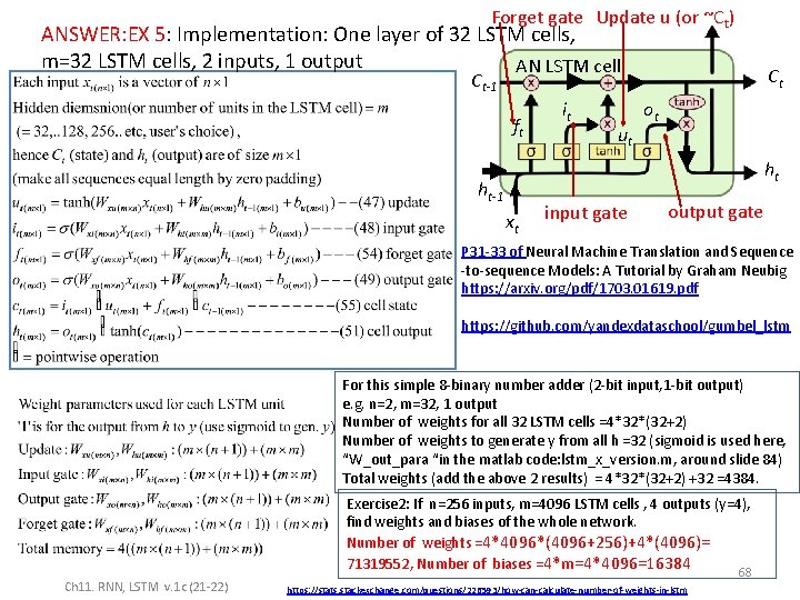
The matrix sizes shown in the formulas and the diagram are for all m duplicated cells . *=elemnt_wise multiplication • Forget gate Ct-1(mx 1) ft(mx 1) i(mx 1) Ct(mx 1) U(mx 1) o (mx 1) t http: //kvitajakub. github. io/2016/04/14/rnndiagrams/ ht(mx 1) X is of size nx 1 h is of size mx 1 ht-1(mx 1) X is of size nx 1 Size( Xt(nx 1) append ht-1(mx 1) )=(n+m)x 1 Ch 11. RNN, LSTM v. 1 c (21 -22) 41

Exercise 2 • In the previous slide, – which part handles long term memory? – which part handles short term memory? Ch 11. RNN, LSTM v. 1 c (21 -22) 42

Answer: 2 – which part handles long term memory? • Answer: C and Forget, input, update output gates – which part handles short term memory? • Answer: Forget, input, update output gates h cell-output for next layer Ct Ct-1 Forget gate Input gate Update gate Output gate ht-1 Input xt Ch 11. RNN, LSTM v. 1 c (21 -22) ht Ch 11. RNN, LSTM 43

Summary of the 7 LSTM equations Wxy are weights ()=sigmoid & tanh()=hyperbolic tangent are activation functions Layer 1 input is from x: The matrix sizes shown in the formulas are for all m duplicated cells Input is nbit Ch 11. RNN, LSTM v. 1 c (21 -22) 44

https: //imiloainf. wordpress. com/2013/11/06/rectifier-nonlinearities/ https: //www. simonwenkel. com/2018/05/15/activation-functions-for-neural-networks. html#softplus Recall : Activation function choices Relu is now very popular and shown to be working better other methods Ch 11. RNN, LSTM v. 1 c (21 -22) 45

LSTM Example Numerical example Ch 11. RNN, LSTM v. 1 c (21 -22) 46

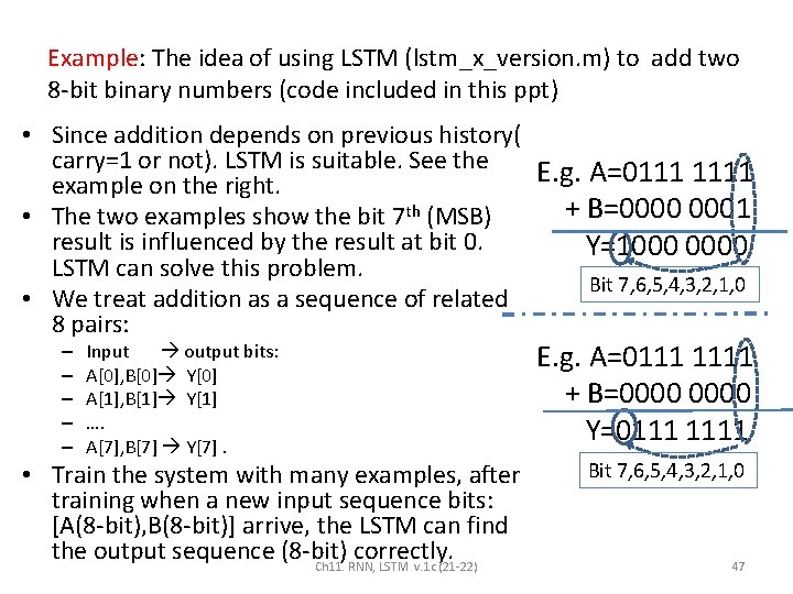
Example: The idea of using LSTM (lstm_x_version. m) to add two 8 -bit binary numbers (code included in this ppt) • Since addition depends on previous history( carry=1 or not). LSTM is suitable. See the E. g. A=0111 1111 example on the right. + B=0000 0001 • The two examples show the bit 7 th (MSB) result is influenced by the result at bit 0. Y=1000 0000 LSTM can solve this problem. Bit 7, 6, 5, 4, 3, 2, 1, 0 • We treat addition as a sequence of related 8 pairs: – – – Input output bits: A[0], B[0] Y[0] A[1], B[1] Y[1] …. A[7], B[7] Y[7]. • Train the system with many examples, after training when a new input sequence bits: [A(8 -bit), B(8 -bit)] arrive, the LSTM can find the output sequence (8 -bit) correctly. Ch 11. RNN, LSTM v. 1 c (21 -22) E. g. A=0111 1111 + B=0000 Y=0111 1111 Bit 7, 6, 5, 4, 3, 2, 1, 0 47

Exercise 3 • In the previous example – Give examples of long term memory is needed – Give examples of short term memory is needed. Ch 11. RNN, LSTM v. 1 c (21 -22) 48

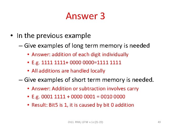
Answer 3 • In the previous example – Give examples of long term memory is needed • Answer: addition of each digit individually • E. g. 1111+ 0000=1111 • All additions are handled locally – Give examples of short term memory is needed. • Answer: Addition or subtraction involves carry • E. g. 0001 1111 + 0000 0001 = 0010 0000 • Result: Bit 5 is 1, it is caused by bit 0 addition Ch 11. RNN, LSTM v. 1 c (21 -22) 49

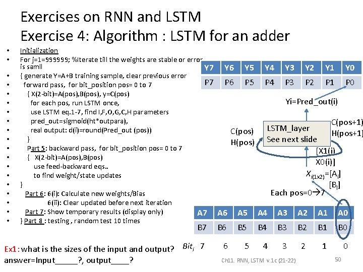
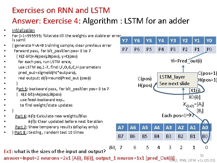
Exercises on RNN and LSTM Exercise 4: Algorithm : LSTM for an adder • • • • • Initialization For j=1=999999; %Iterate till the weights are stable or error is samll Y 7 { generate Y=A+B training sample, clear previous error P 7 forward pass, for bit_position pos= 0 to 7 { X(2 -bit)=A(pos), B(pos), y=C(pos) for each pos, run LSTM once, use LSTM eq. 1 -7, find I, F, O, G, C, H parameters pred_out=sigmoid(ht*outpara), real output: d(i)=round(Pred_out (pos)) } Part 5: backward pass, for bit_position pos= 0 to 7 { X(2 -bit)=A(pos), B(pos) use feed-backward eqs. . to find weight/state updates } Part 6: 6(i): Calculate new weights/Bias 6(ii): Clear updated before next iteration Part 7: Show temporary results (display only) A 7 } Part 8 : testing , random test 10 times Y 6 Y 5 Y 4 Y 3 Y 2 Y 1 Y 0 P 6 P 5 P 4 P 3 P 2 P 1 P 0 Yi=Pred_out(i) C(pos) H(pos) C(pos+1) LSTM_layer H(pos+1) See next slide [X 1(i) X 0(i)] Xi(1 x 2)=[Ai] [Bi] Each pos=0 7 A 6 A 5 A 4 A 3 A 2 A 1 A 0 B 7 B 6 B 5 B 4 B 3 B 2 B 1 B 0 Ex 1: what is the sizes of the input and output? Biti 7 answer=Input_____? , output____? 6 5 4 3 2 1 0 Ch 11. RNN, LSTM v. 1 c (21 -22) 50

Exercises on RNN and LSTM Answer: Exercise 4: Algorithm : LSTM for an adder • • • • • Initialization For j=1=999999; %Iterate till the weights are stable or error is samll Y 7 { generate Y=A+B training sample, clear previous error P 7 forward pass, for bit_position pos= 0 to 7 { X(2 -bit)=A(pos), B(pos), y=C(pos) for each pos, run LSTM once, use LSTM eq. 1 -7, find I, F, O, G, C, H parameters pred_out=sigmoid(ht*outpara), real output: d(i)=round(Pred_out (pos)) } Part 5: backward pass, for bit_position pos= 0 to 7 { X(2 -bit)=A(pos), B(pos) use feed-backward eqs. . to find weight/state updates } Part 6: 6(i): Calculate new weights/Bias 6(ii): Clear updated before next iteration Part 7: Show temporary results (display only) A 7 } Part 8 : testing , random test 10 times Y 6 Y 5 Y 4 Y 3 Y 2 Y 1 Y 0 P 6 P 5 P 4 P 3 P 2 P 1 P 0 Yi=Pred_out(i) C(pos) H(pos) C(pos+1) LSTM_layer H(pos+1) See next slide [X 1(i) X 0(i)] Xi(1 x 2)=[Ai] [Bi] Each pos=0 7 A 6 A 5 A 4 A 3 A 2 A 1 A 0 B 6 B 5 B 4 B 3 B 2 B 1 B 0 Biti 7 6 5 4 3 2 1 Ex 1: what is the sizes of the input and output? answer=Input=2 neurons =2 x 1 [A(i), B(i)], output_1 neuron =1 x 1 [pred_Out(i)] Ch 11. RNN, LSTM 0 B 7 51 v. 1 c (21 -22)

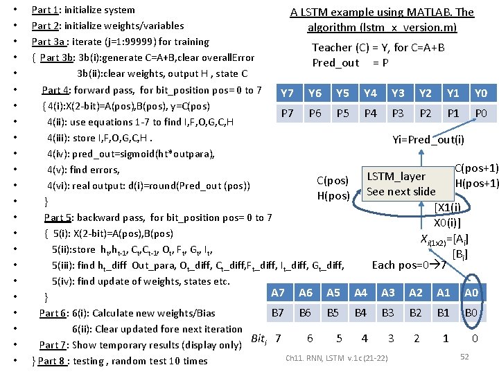
• • • • • • Part 1: initialize system A LSTM example using MATLAB. The Part 2: initialize weights/variables algorithm (lstm_x_version. m) Part 3 a : iterate (j=1: 99999) for training Teacher (C) = Y, for C=A+B { Part 3 b: 3 b(i): generate C=A+B, clear overall. Error Pred_out = P 3 b(ii): clear weights, output H , state C Part 4: forward pass, for bit_position pos= 0 to 7 Y 6 Y 5 Y 4 Y 3 Y 2 Y 1 Y 0 { 4(i): X(2 -bit)=A(pos), B(pos), y=C(pos) P 7 P 6 P 5 P 4 P 3 P 2 P 1 P 0 4(ii): use equations 1 -7 to find I, F, O, G, C, H 4(iii): store I, F, O, G, C, H. Yi=Pred_out(i) 4(iv): pred_out=sigmoid(ht*outpara), C(pos+1) 4(v): find errors, LSTM_layer C(pos) H(pos+1) 4(vi): real output: d(i)=round(Pred_out (pos)) See next slide H(pos) } [X 1(i) Part 5: backward pass, for bit_position pos= 0 to 7 X 0(i)] { 5(i): X(2 -bit)=A(pos), B(pos) Xi(1 x 2)=[Ai] 5(ii): store ht, ht-1, Ct-1, Ot, Ft, Gt, It, [Bi] 5(iii): find ht_diff Out_para, Ot_diff, Ct_diff, Ft_diff, It_diff, Gt_diff, Each pos=0 7 5(iv): find update of weights, states etc. A 7 A 6 A 5 A 4 A 3 A 2 A 1 A 0 } Part 6: 6(i): Calculate new weights/Bias B 7 B 6 B 5 B 4 B 3 B 2 B 1 B 0 6(ii): Clear updated fore next iteration Biti 7 6 5 4 3 2 1 0 Part 7: Show temporary results (display only) 52 Ch 11. RNN, LSTM v. 1 c (21 -22) } Part 8 : testing , random test 10 times

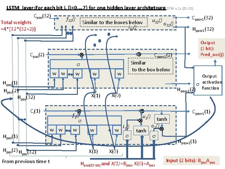
LSTM_layer: For each bit j, (j=0, . . , 7) for one hidden layer architetcure Ch 11. RNN, LSTM Cpos(32) f 32() u 32() Total weights Similar to the boxes below o 32() i () 32 =4*[32*(32+2)] w w Hpos(1) Hpos(2) Hpos(32) X(1) Hpos(2) H (32) pos From previous time t w w w X(1) w Hpos+1(32) Output (1 bit): Pred_out(j) Output activation Hpos+1(2) function X(0) f 1() Ci(1) Cpos+1(32) Cpos+1(2) Similar to the box below Cpos(2) v. 1 c (21 -22) I 1() u 1() tanh o 1() tanh X(0) Hpos(32 -bit) and X(1)=Bpos, X(0)=Apos Cpos+1(1) Hpos+1(1) • 53 Input (2 bits): Bpos. Apos

Recall: Hierarchical structure of a form of stacked LSTM Real Output (y) output neurons • n inputs (X) • M layers – i-th layer has mi cells, (i=1, 2, . . , M) Output activation function, e. g. sigmoid( ) or softmax h LSTM Layer M, m. M cells • y real output neurons. • The “Output activation function” can be sigmoid or softmax • Initialize h(t=0), C(t=0)=zeros h LSTM Layer 2, m 2 cells h LSTM Layer h 1, m 1 cells t t+1 {X(1) , X(2), …, X(n)}t Ch 11. RNN, LSTM v. 1 c (21 -22) 54 https: //towardsdatascience. com/implementation-of-rnn-lstm-and-gru-a 4250 bf 6 c 090

Recall : From input to layer 1 A cell has 4 components Ct-1(mi, i) From Previous cycle C (t-1) ht-1 Previous time Ct (mi, i) Cell mi Ct-1(2, i) ht(mi, i) Cell 2 Ct-1(1, i) ht Next layer Cell 1 Ct (2, i) ht(2, i) C (t+1) Ct (1, i) ht(1, i) If this is the first layer Inputs {x 1, x 2, …, xn}t, , input has n bits Ch 11. RNN, LSTM v. 1 c (21 -22) 55 https: //towardsdatascience. com/implementation-of-rnn-lstm-and-gru-a 4250 bf 6 c 090

Recall : From hidden ith layer to i+1 th layer A cell has 4 components Ct-1(mi, i) From Previous cycle C (t-1) ht-1 Previous time Ct (mi, i) Cell mi Ct-1(2, i) ht(mi, i) Cell 2 Ct-1(1, i) ht Next layer Cell 1 Ct (2, i) ht(2, i) C (t+1) Ct (1, i) ht(1, i) If this is the ith hidden layer, input is from i-1 th layer Assume in this ith layer, there are mi cells The previous layer has mi-1 cells Ch 11. RNN, LSTM v. 1 c (21 -22) 56 https: //towardsdatascience. com/implementation-of-rnn-lstm-and-gru-a 4250 bf 6 c 090

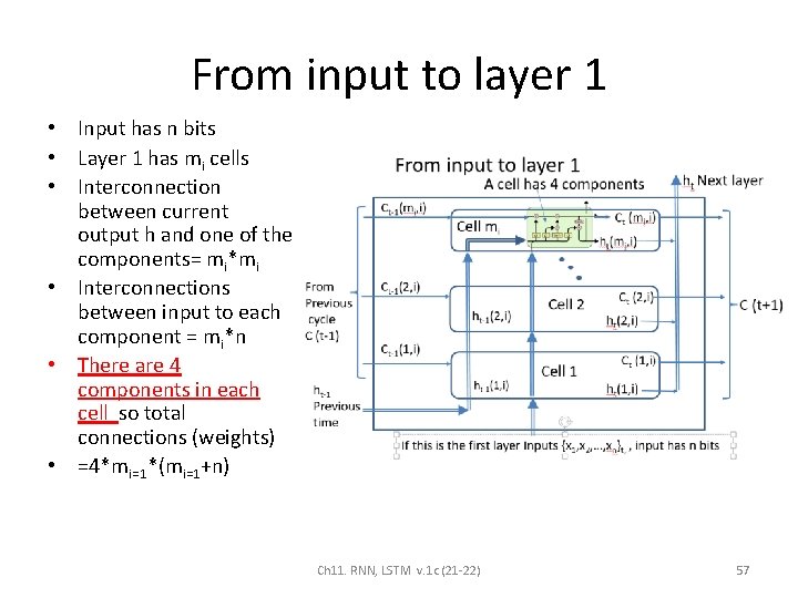
From input to layer 1 • Input has n bits • Layer 1 has mi cells • Interconnection between current output h and one of the components= mi*mi • Interconnections between input to each component = mi*n • There are 4 components in each cell so total connections (weights) • =4*mi=1*(mi=1+n) Ch 11. RNN, LSTM v. 1 c (21 -22) 57

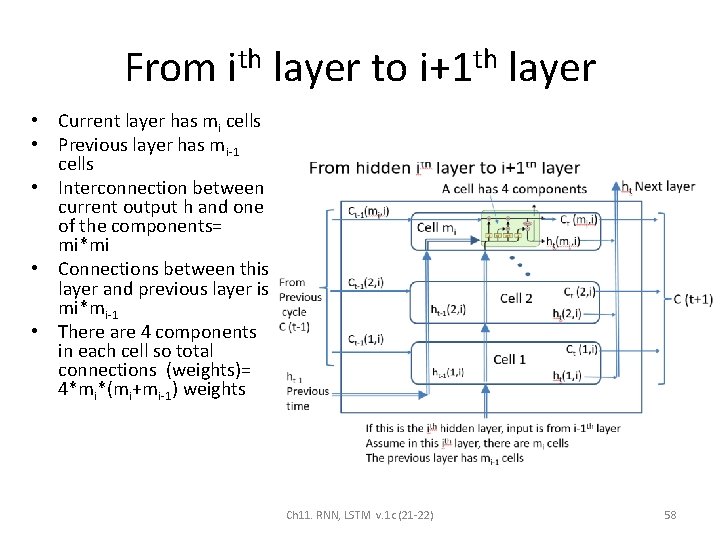
From ith layer to i+1 th layer • Current layer has mi cells • Previous layer has mi-1 cells • Interconnection between current output h and one of the components= mi*mi • Connections between this layer and previous layer is mi*mi-1 • There are 4 components in each cell so total connections (weights)= 4*mi*(mi+mi-1) weights Ch 11. RNN, LSTM v. 1 c (21 -22) 58

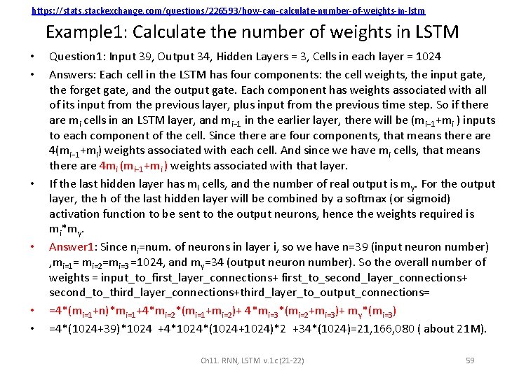
https: //stats. stackexchange. com/questions/226593/how-can-calculate-number-of-weights-in-lstm Example 1: Calculate the number of weights in LSTM • • • Question 1: Input 39, Output 34, Hidden Layers = 3, Cells in each layer = 1024 Answers: Each cell in the LSTM has four components: the cell weights, the input gate, the forget gate, and the output gate. Each component has weights associated with all of its input from the previous layer, plus input from the previous time step. So if there are mi cells in an LSTM layer, and mi− 1 in the earlier layer, there will be (mi− 1+mi ) inputs to each component of the cell. Since there are four components, that means there are 4(mi− 1+mi) weights associated with each cell. And since we have mi cells, that means there are 4 mi (mi− 1+mi ) weights associated with that layer. If the last hidden layer has mi cells, and the number of real output is my. For the output layer, the h of the last hidden layer will be combined by a softmax (or sigmoid) activation function to be sent to the output neurons, hence the weights required is mi*my. Answer 1: Since ni=num. of neurons in layer i, so we have n=39 (input neuron number) , mi=1= mi=2=mi=3 =1024, and my=34 (output neuron number). So the overall number of weights = input_to_first_layer_connections+ first_to_second_layer_connections+ second_to_third_layer_connections+third_layer_to_output_connections= =4*(mi=1+n)*mi=1+4*mi=2*(mi=1+mi=2)+ 4*mi=3*(mi=2+mi=3)+ my*(mi=3) =4*(1024+39)*1024 +4*1024*(1024+1024)*2 +34*(1024)=21, 166, 080 ( about 21 M). Ch 11. RNN, LSTM v. 1 c (21 -22) 59

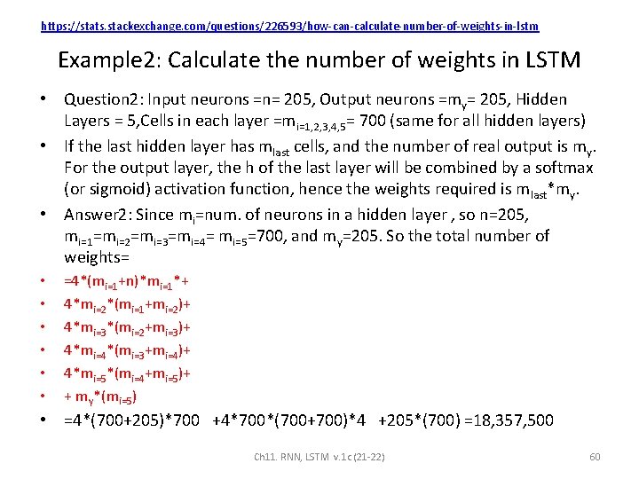
https: //stats. stackexchange. com/questions/226593/how-can-calculate-number-of-weights-in-lstm Example 2: Calculate the number of weights in LSTM • Question 2: Input neurons =n= 205, Output neurons =my= 205, Hidden Layers = 5, Cells in each layer =mi=1, 2, 3, 4, 5= 700 (same for all hidden layers) • If the last hidden layer has mlast cells, and the number of real output is my. For the output layer, the h of the last layer will be combined by a softmax (or sigmoid) activation function, hence the weights required is mlast*my. • Answer 2: Since mi=num. of neurons in a hidden layer , so n=205, mi=1=mi=2=mi=3=mi=4= mi=5=700, and my=205. So the total number of weights= • =4*(mi=1+n)*mi=1*+ • • • 4*mi=2*(mi=1+mi=2)+ 4*mi=3*(mi=2+mi=3)+ 4*mi=4*(mi=3+mi=4)+ 4*mi=5*(mi=4+mi=5)+ + my*(mi=5) • =4*(700+205)*700 +4*700*(700+700)*4 +205*(700) =18, 357, 500 Ch 11. RNN, LSTM v. 1 c (21 -22) 60

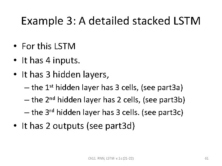
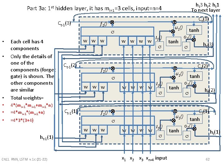
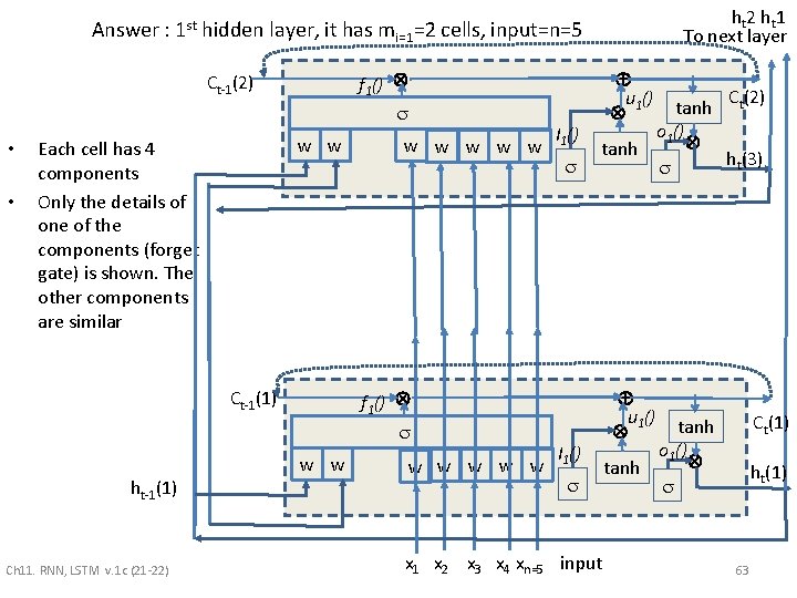
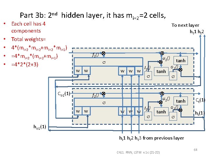
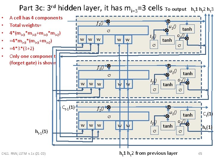
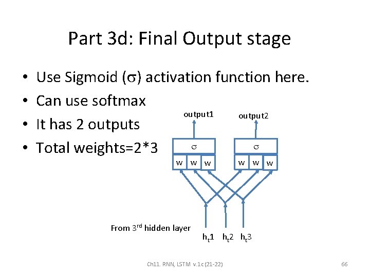
Example 3: A detailed stacked LSTM • For this LSTM • It has 4 inputs. • It has 3 hidden layers, – the 1 st hidden layer has 3 cells, (see part 3 a) – the 2 nd hidden layer has 2 cells, (see part 3 b) – the 3 rd hidden layer has 3 cells. (see part 3 c) • It has 2 outputs (see part 3 d) Ch 11. RNN, LSTM v. 1 c (21 -22) 61

ht 3 h t 2 h t 1 To next layer Part 3 a: 1 st hidden layer, it has mi=1=3 cells, input=n=4 Ct-1(3) • Each cell has 4 components Only the details of one of the components (forget gate) is shown. The other components are similar Total weights= • • 4*(mi=1*mi=1+mi=1*n) =4*mi=1*(mi=1+n) • =4*3*(3+4) • • f 1() w w w Ct-1(2) f 1() w w w Ct-1(1) Ch 11. RNN, LSTM v. 1 c (21 -22) w w f 1() w w w ht-1(1) w w w w I 1() x 1 x 2 x 3 xn=4 input u 1() Ct(3) tanh o 1() tanh ht(3) u 1() Ct(2) tanh o 1() tanh ht(2) Ct(1) tanh o 1() tanh ht(1) u 1() 62

ht 2 h t 1 To next layer Answer : 1 st hidden layer, it has mi=1=2 cells, input=n=5 f 1() Ct-1(2) • • w w Each cell has 4 components Only the details of one of the components (forget gate) is shown. The other components are similar f 1() Ct-1(1) ht-1(1) Ch 11. RNN, LSTM v. 1 c (21 -22) w w w I 1() u 1() C (2) tanh t o 1() tanh ht(3) I 1() x 1 x 2 x 3 x 4 xn=5 input u 1() Ct(1) tanh o 1() tanh ht(1) 63

Part 3 b: 2 nd hidden layer, it has mi=2=2 cells, • Each cell has 4 components • Total weights= • 4*(mi=2*mi=2+mi=2*mi=1) • =4*mi=2*(mi=2+mi=1) • =4*2*(2+3) To next layer ht 1 h t 2 f 1() w w w f 1() Ct-1(1) w w w I 1() u 1() tanh o 1() tanh Ct(1) ht-1(1) ht 1 ht 2 ht 3 from previous layer Ch 11. RNN, LSTM v. 1 c (21 -22) 64

Part 3 c: 3 rd hidden layer, it has mi=3=3 cells To output • • • A cell has 4 components Total weights= 4*(mi=3*mi=3+mi=3*mi=2) =4*mi=3*(mi=3+mi=2) =4*3*(3+2) Only one component (forget gate) is shown f 1() w w w Ct-1(1) ht-1(1) Ch 11. RNN, LSTM v. 1 c (21 -22) w w f 1() w w w I 1() ht 1 h t 2 h t 3 u 1() tanh o 1() tanh u 1() Ct(1) tanh o 1() tanh ht 1 ht 2 from previous layer ht(1) 65

Part 3 d: Final Output stage • • Use Sigmoid ( ) activation function here. Can use softmax output 1 output 2 It has 2 outputs Total weights=2*3 w w w From 3 rd hidden layer w w w ht 1 h t 2 h t 3 Ch 11. RNN, LSTM v. 1 c (21 -22) 66

Forget gate Update u (or ~Ct) Exercise 5: Implementation: One layer of 32 LSTM cells, m=32 LSTM cells, 2 inputs, 1 output AN LSTM cell Ct Ct-1 ft it ut ot ht ht-1 xt input gate output gate P 31 -33 of Neural Machine Translation and Sequence -to-sequence Models: A Tutorial by Graham Neubig https: //arxiv. org/pdf/1703. 01619. pdf https: //github. com/yandexdataschool/gumbel_lstm For this simple 8 -binary number adder (2 -bit input, 1 -bit output) e. g. n=2, m=32, 1 output Number of weights for all 32 LSTM cells =4*32*(32+2) Number of weights to generate y from all h =32 (sigmoid is used here, “W_out_para “in the matlab code: lstm_x_version. m, around slide 84) Total weights (add the above 2 results) = 4*32*(32+2) +32 =4384. Ch 11. RNN, LSTM v. 1 c (21 -22) Exercise 2: If n=256 inputs, m=4096 LSTM cells , 4 outputs (y=4), find weights and biases of the whole network. Number of weights =_______? Number of biases =________? 67 http: //www. 4 answered. com/questions/view/2450 e 23/How-to-calculate-the-number-of-parameters-of-an-LSTM-network

Forget gate Update u (or ~Ct) ANSWER: EX 5: Implementation: One layer of 32 LSTM cells, m=32 LSTM cells, 2 inputs, 1 output AN LSTM cell Ct Ct-1 ft it ut ot ht ht-1 xt input gate output gate P 31 -33 of Neural Machine Translation and Sequence -to-sequence Models: A Tutorial by Graham Neubig https: //arxiv. org/pdf/1703. 01619. pdf https: //github. com/yandexdataschool/gumbel_lstm For this simple 8 -binary number adder (2 -bit input, 1 -bit output) e. g. n=2, m=32, 1 output Number of weights for all 32 LSTM cells =4*32*(32+2) Number of weights to generate y from all h =32 (sigmoid is used here, “W_out_para “in the matlab code: lstm_x_version. m, around slide 84) Total weights (add the above 2 results) = 4*32*(32+2) +32 =4384. Ch 11. RNN, LSTM v. 1 c (21 -22) Exercise 2: If n=256 inputs, m=4096 LSTM cells , 4 outputs (y=4), find weights and biases of the whole network. Number of weights =4*4096*(4096+256)+4*(4096)= 71319552, Number of biases =4*m=4*4096=16384 68 https: //stats. stackexchange. com/questions/226593/how-can-calculate-number-of-weights-in-lstm

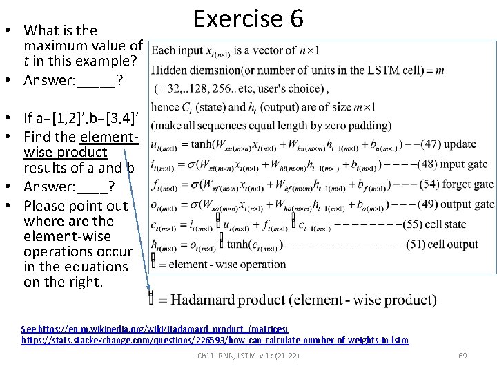
• What is the maximum value of t in this example? • Answer: _____? Exercise 6 • If a=[1, 2]’, b=[3, 4]’ • Find the elementwise product results of a and b • Answer: ____? • Please point out where are the element-wise operations occur in the equations on the right. See https: //en. m. wikipedia. org/wiki/Hadamard_product_(matrices) https: //stats. stackexchange. com/questions/226593/how-can-calculate-number-of-weights-in-lstm Ch 11. RNN, LSTM v. 1 c (21 -22) 69

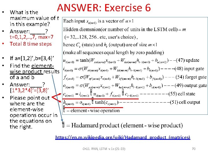
ANSWER: Exercise 6 • What is the maximum value of t in this example? • Answer: _____? t=0, 1, 2, . . , 7, max=7 • Total 8 time steps • If a=[1, 2]’, b=[3, 4]’ • Find the elementwise product results of a and b • Answer: ____? [1*3, 2*4]’=[3, 8]’ • Please point out where are the element-wise operations occur in the equations on the right. https: //en. m. wikipedia. org/wiki/Hadamard_product_(matrices) Ch 11. RNN, LSTM v. 1 c (21 -22) 70

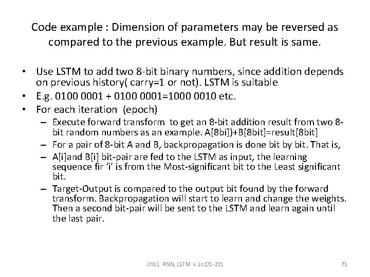
Code example : Dimension of parameters may be reversed as compared to the previous example. But result is same. • Use LSTM to add two 8 -bit binary numbers, since addition depends on previous history( carry=1 or not). LSTM is suitable • E. g. 0100 0001 + 0100 0001=1000 0010 etc. • For each iteration (epoch) – Execute forward transform to get an 8 -bit addition result from two 8 bit random numbers as an example. A[8 bi])+B[8 bit]=result[8 bit] – For a pair of 8 -bit A and B, backpropagation is done bit by bit. That is, – A[i]and B[i] bit-pair are fed to the LSTM as input, the learning sequence fir ‘i’ is from the Most-significant bit to the Least significant bit. – Target-Output is compared to the output bit found by the forward transform. Backpropagation will start to learn and change the weights. Then a second bit-pair will be sent to the LSTM and learn again until the last pair. Ch 11. RNN, LSTM v. 1 c (21 -22) 71

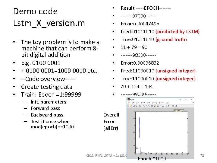
Demo code Lstm_X_version. m • The toy problem is to make a machine that can perform 8 bit digital addition • E. g. 0100 0001 • + 0100 0001=1000 0010 etc. • --Code overview---- • Create testing data • Train: Epoch =1: 99999 – – Init. parameters Forward pass Backward pass Test it once when mod(epoch)==1000 • • • Result -----EPOCH-------97000 -----Error: 0. 00047496 Pred: 01011010 (predicted by LSTM) True: 01011010 (ground truth) 11 + 79 = 90 -------98000 -----Error: 0. 00036832 Pred: 11000010 (unsigned integer) True: 11000010 (unsigned integer) 70 + 124 = 194 -------99000 ------ Overall Error (all. Err) Ch 11. RNN, LSTM v. 1 c (21 -22) Epoch *1000 72

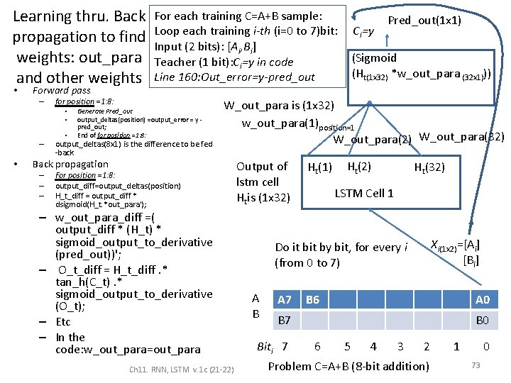
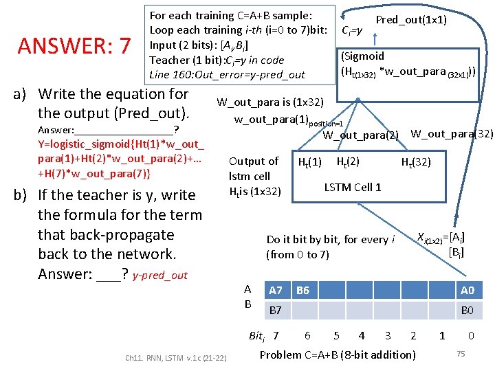
Learning thru. Back propagation to find weights: out_para and other weights • Forward pass – for position =1: 8: • • • – • For each training C=A+B sample: Loop each training i-th (i=0 to 7)bit: Input (2 bits): [Ai, Bi] Teacher (1 bit): Ci=y in code Line 160: Out_error=y-pred_out Generate Pred_out output_deltas(position) =output_error = y pred_out; End of for position =1: 8: output_deltas(8 x 1) is the difference to be fed -back (Sigmoid (Ht(1 x 32) *w_out_para (32 x 1))) W_out_para is (1 x 32) w_out_para(1)position=1 W_out_para(2) W_out_para(32) Back propagation – – – Ci=y Pred_out(1 x 1) For position =1: 8: output_diff=output_deltas(position) H_t_diff = output_diff * dsigmoid(H_t. *out_para'); – w_out_para_diff =( output_diff * (H_t) * sigmoid_output_to_derivative (pred_out))'; – O_t_diff = H_t_diff. * tan_h(C_t). * sigmoid_output_to_derivative (O_t); – Etc – In the code: w_out_para=out_para Ch 11. RNN, LSTM v. 1 c (21 -22) Output of lstm cell Htis (1 x 32) Ht(1) Ht(2) Ht(32) LSTM Cell 1 Xi(1 x 2)=[Ai] [Bi] Do it by bit, for every i (from 0 to 7) A B A 7 B 6 A 0 B 7 Biti 7 B 0 6 5 4 3 2 Problem C=A+B (8 -bit addition) 1 0 73

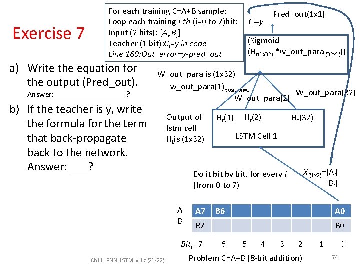
Exercise 7 For each training C=A+B sample: Loop each training i-th (i=0 to 7)bit: Input (2 bits): [Ai, Bi] Teacher (1 bit): Ci=y in code Line 160: Out_error=y-pred_out a) Write the equation for the output (Pred_out). Answer: _________? b) If the teacher is y, write the formula for the term that back-propagate back to the network. Answer: ___? Ci=y Pred_out(1 x 1) (Sigmoid (Ht(1 x 32) *w_out_para (32 x 1))) W_out_para is (1 x 32) w_out_para(1)position=1 W_out_para(32) W_out_para(2) Output of lstm cell Htis (1 x 32) Ht(32) LSTM Cell 1 Xi(1 x 2)=[Ai] [Bi] Do it by bit, for every i (from 0 to 7) A B A 7 B 6 A 0 B 7 Biti 7 Ch 11. RNN, LSTM v. 1 c (21 -22) Ht(1) B 0 6 5 4 3 2 Problem C=A+B (8 -bit addition) 1 0 74

ANSWER: 7 For each training C=A+B sample: Loop each training i-th (i=0 to 7)bit: Input (2 bits): [Ai, Bi] Teacher (1 bit): Ci=y in code Line 160: Out_error=y-pred_out a) Write the equation for the output (Pred_out). Answer: _________? Y=logistic_sigmoid{Ht(1)*w_out_ para(1)+Ht(2)*w_out_para(2)+… +H(7)*w_out_para(7)} Ci=y Pred_out(1 x 1) (Sigmoid (Ht(1 x 32) *w_out_para (32 x 1))) W_out_para is (1 x 32) w_out_para(1)position=1 W_out_para(2) W_out_para(32) b) If the teacher is y, write the formula for the term that back-propagate back to the network. Answer: ___? y-pred_out Output of lstm cell Htis (1 x 32) Ht(32) LSTM Cell 1 Xi(1 x 2)=[Ai] [Bi] Do it by bit, for every i (from 0 to 7) A B A 7 B 6 A 0 B 7 Biti 7 Ch 11. RNN, LSTM v. 1 c (21 -22) Ht(1) B 0 6 5 4 3 2 Problem C=A+B (8 -bit addition) 1 0 75

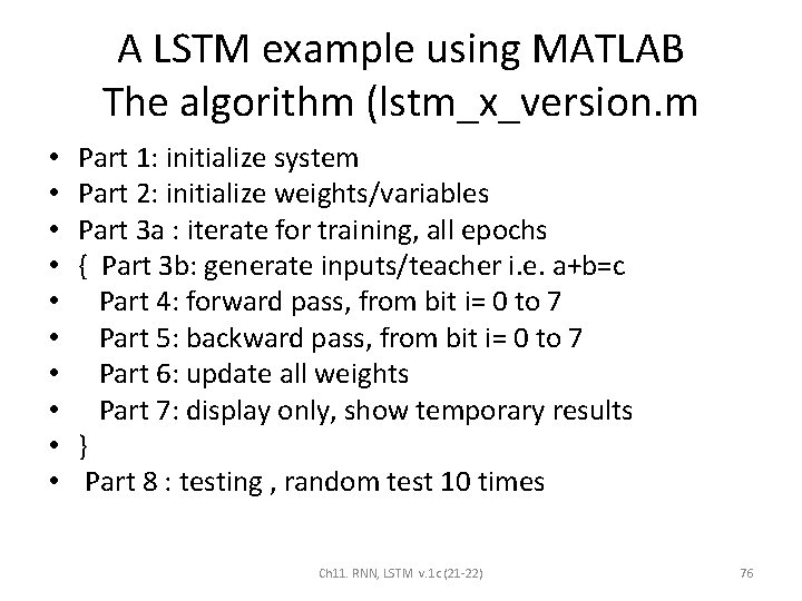
A LSTM example using MATLAB The algorithm (lstm_x_version. m • • • Part 1: initialize system Part 2: initialize weights/variables Part 3 a : iterate for training, all epochs { Part 3 b: generate inputs/teacher i. e. a+b=c Part 4: forward pass, from bit i= 0 to 7 Part 5: backward pass, from bit i= 0 to 7 Part 6: update all weights Part 7: display only, show temporary results } Part 8 : testing , random test 10 times Ch 11. RNN, LSTM v. 1 c (21 -22) 76

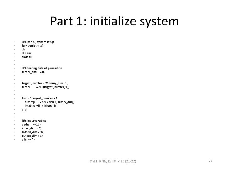
Part 1: initialize system • • • • • • • %% part 1 , system setup function lstm_x() clc % clear close all %% training dataset generation binary_dim = 8; largest_number = 2^binary_dim - 1; binary = cell(largest_number, 1); for i = 1: largest_number + 1 binary{i} = dec 2 bin(i-1, binary_dim); int 2 binary{i} = binary{i}; end %% input variables alpha = 0. 1; input_dim = 2; hidden_dim = 32; output_dim = 1; all. Err = []; Ch 11. RNN, LSTM v. 1 c (21 -22) 77

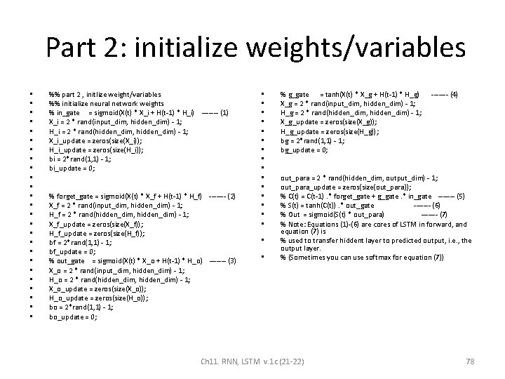
Part 2: initialize weights/variables • • • • • • • %% part 2 , initlize weight/variables %% initialize neural network weights % in_gate = sigmoid(X(t) * X_i + H(t-1) * H_i) ------- (1) X_i = 2 * rand(input_dim, hidden_dim) - 1; H_i = 2 * rand(hidden_dim, hidden_dim) - 1; X_i_update = zeros(size(X_i)); H_i_update = zeros(size(H_i)); bi = 2*rand(1, 1) - 1; bi_update = 0; % forget_gate = sigmoid(X(t) * X_f + H(t-1) * H_f) ------- (2) X_f = 2 * rand(input_dim, hidden_dim) - 1; H_f = 2 * rand(hidden_dim, hidden_dim) - 1; X_f_update = zeros(size(X_f)); H_f_update = zeros(size(H_f)); bf = 2*rand(1, 1) - 1; bf_update = 0; % out_gate = sigmoid(X(t) * X_o + H(t-1) * H_o) ------- (3) X_o = 2 * rand(input_dim, hidden_dim) - 1; H_o = 2 * rand(hidden_dim, hidden_dim) - 1; X_o_update = zeros(size(X_o)); H_o_update = zeros(size(H_o)); bo = 2*rand(1, 1) - 1; bo_update = 0; • • • • • % g_gate = tanh(X(t) * X_g + H(t-1) * H_g) X_g = 2 * rand(input_dim, hidden_dim) - 1; H_g = 2 * rand(hidden_dim, hidden_dim) - 1; X_g_update = zeros(size(X_g)); H_g_update = zeros(size(H_g)); bg = 2*rand(1, 1) - 1; bg_update = 0; ------- (4) out_para = 2 * rand(hidden_dim, output_dim) - 1; out_para_update = zeros(size(out_para)); % C(t) = C(t-1). * forget_gate + g_gate. * in_gate ------- (5) % S(t) = tanh(C(t)). * out_gate ------- (6) % Out = sigmoid(S(t) * out_para) ------- (7) % Note: Equations (1)-(6) are cores of LSTM in forward, and equation (7) is % used to transfer hiddent layer to predicted output, i. e. , the output layer. % (Sometimes you can use softmax for equation (7)) Ch 11. RNN, LSTM v. 1 c (21 -22) 78

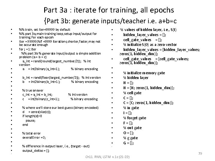
Part 3 a : iterate for training, all epochs {Part 3 b: generate inputs/teacher i. e. a+b=c • • • • • • • %% train, set iter=99999 by default %% part 3 a, main training loop, setup input/output for training. For each epcoh iter = 99999; %if =9999 iterations, shorter, faster, may not be accurate enough for j = 1: iter %% part 3 b % generate input/output a simple addition problem (a + b = c) a_int = randi(round(largest_number/2)); % int version a = int 2 binary{a_int+1}; % binary encoding b_int = randi(floor(largest_number/2)); % int version b = int 2 binary{b_int+1}; % binary encoding % true answer c_int = a_int + b_int; c = int 2 binary{c_int+1}; % int version % binary encoding % where we'll store our best guess (binary encoded) d = zeros(size(c)); if length(d)<8 pause; end % total error overall. Error = 0; % difference in output layer, i. e. , (target - out) output_deltas = []; • • • • • • % values of hidden layer, i. e. , S(t) hidden_layer_values = []; cell_gate_values = []; % initialize S(0) as a zero-vector hidden_layer_values = [hidden_layer_values; zeros(1, hidden_dim)]; cell_gate_values = [cell_gate_values; zeros(1, hidden_dim)]; % initialize memory gate % hidden layer H = []; H = [H; zeros(1, hidden_dim)]; % cell gate C = []; C = [C; zeros(1, hidden_dim)]; % in gate I = []; % forget gate F = []; % out gate O = []; % g gate G = []; Ch 11. RNN, LSTM v. 1 c (21 -22) 79

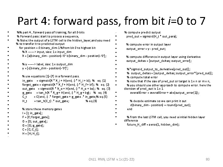
Part 4: forward pass, from bit i=0 to 7 • • • • • • • %% part 4 , forward pass of training, for all 8 -bits % Forward pass: start to process a sequence, % Note: the output of a LSTM cell is the hidden_layer, and you need % to transfer it to predicted output for position = 0: binary_dim-1 %from bit 0 to highest bit % X ------> input, size: 1 x input_dim X = [a(binary_dim - position)-'0' b(binary_dim - position)-'0']; % y ------> label, size: 1 x output_dim y = [c(binary_dim - position)-'0']'; % use equations (1)-(7) in a forward pass. in_gate = sigmoid(X * X_i + H(end, : ) * H_i + bi); % eq. (1) forget_gate = sigmoid(X * X_f + H(end, : ) * H_f + bf); % eq. (2) out_gate = sigmoid(X * X_o + H(end, : ) * H_o + bo); % eq. (3) g_gate = tan_h(X * X_g + H(end, : ) * H_g + bg); % eq. (4) C_t = C(end, : ). * forget_gate + g_gate. * in_gate; % eq. (5) H_t = tan_h(C_t). * out_gate; % eq. (6) % store these memory gates I = [I; in_gate]; F = [F; forget_gate]; O = [O; out_gate]; G = [G; g_gate]; C = [C; C_t]; H = [H; H_t]; • • • • • • % compute predict output pred_out = sigmoid(H_t * out_para); % compute error in output layer output_error = y - pred_out; % compute difference in output layer using derivative output_deltas = [output_deltas; output_error]; %*sigmoid_output_to_derivative(pred_out)]; % output_deltas = [output_deltas; output_error*(pred_out)]; % compute total error % note that if the size of pred_out or target is 1 x n or m x n, % you should use other approach to compute error. here the diension of pred_out is 1 x 1 overall. Error = overall. Error + abs(output_error(1)); % decode estimate so we can print it out d(binary_dim - position) = round(pred_out); end % from the last LSTM cell, you need a initial hidden layer difference future_H_diff = zeros(1, hidden_dim); Ch 11. RNN, LSTM v. 1 c (21 -22) 80

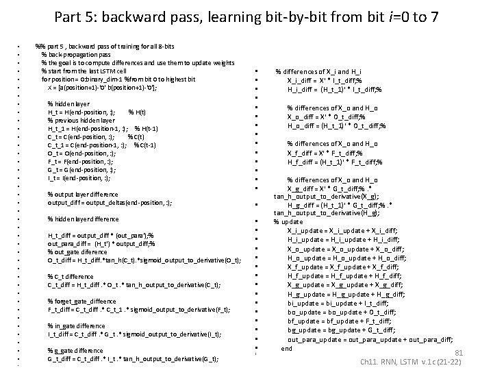
Part 5: backward pass, learning bit-by-bit from bit i=0 to 7 • • • • • • • • • • %% part 5 , backward pass of training for all 8 -bits % back-propagation pass % the goal is to compute differences and use them to update weights % start from the last LSTM cell for position = 0: binary_dim-1 %from bit 0 to highest bit X = [a(position+1)-'0' b(position+1)-'0']; % hidden layer H_t = H(end-position, : ); % H(t) % previous hidden layer H_t_1 = H(end-position-1, : ); % H(t-1) C_t = C(end-position, : ); % C(t) C_t_1 = C(end-position-1, : ); % C(t-1) O_t = O(end-position, : ); F_t = F(end-position, : ); G_t = G(end-position, : ); I_t = I(end-position, : ); % output layer difference output_diff = output_deltas(end-position, : ); % hidden layer difference H_t_diff = output_diff * (out_para'); % out_para_diff = (H_t') * output_diff; % % out_gate diference O_t_diff = H_t_diff. *tan_h(C_t). *sigmoid_output_to_derivative(O_t); % C_t difference C_t_diff = H_t_diff. * O_t. * tan_h_output_to_derivative(C_t); % forget_gate_diffeence F_t_diff = C_t_diff. * C_t_1. * sigmoid_output_to_derivative(F_t); % in_gate difference I_t_diff = C_t_diff. * G_t. * sigmoid_output_to_derivative(I_t); % g_gate difference G_t_diff = C_t_diff. * I_t. * tan_h_output_to_derivative(G_t); • • • • • • • • % differences of X_i and H_i X_i_diff = X' * I_t_diff; % H_i_diff = (H_t_1)' * I_t_diff; % % differences of X_o and H_o X_o_diff = X' * O_t_diff; % H_o_diff = (H_t_1)' * O_t_diff; % % differences of X_o and H_o X_f_diff = X' * F_t_diff; % H_f_diff = (H_t_1)' * F_t_diff; % % differences of X_o and H_o X_g_diff = X' * G_t_diff; %. * tan_h_output_to_derivative(X_g); H_g_diff = (H_t_1)' * G_t_diff; %. * tan_h_output_to_derivative(H_g); % update X_i_update = X_i_update + X_i_diff; H_i_update = H_i_update + H_i_diff; X_o_update = X_o_update + X_o_diff; H_o_update = H_o_update + H_o_diff; X_f_update = X_f_update + X_f_diff; H_f_update = H_f_update + H_f_diff; X_g_update = X_g_update + X_g_diff; H_g_update = H_g_update + H_g_diff; bi_update = bi_update + I_t_diff; bo_update = bo_update + O_t_diff; bf_update = bf_update + F_t_diff; bg_update = bg_update + G_t_diff; out_para_update = out_para_update + out_para_diff; end 81 Ch 11. RNN, LSTM v. 1 c (21 -22)

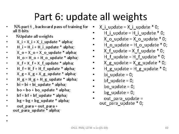
Part 6: update all weights • • • • %% part 6 , backward pass of training for all 8 -bits %Update all weights X_i = X_i + X_i_update * alpha; H_i = H_i + H_i_update * alpha; X_o = X_o + X_o_update * alpha; H_o = H_o + H_o_update * alpha; X_f = X_f + X_f_update * alpha; H_f = H_f + H_f_update * alpha; X_g = X_g + X_g_update * alpha; H_g = H_g + H_g_update * alpha; bi = bi + bi_update * alpha; bo = bo + bo_update * alpha; bf = bf + bf_update * alpha; bg = bg + bg_update * alpha; out_para = out_para + out_para_update * alpha; • X_i_update = X_i_update * 0; • H_i_update = H_i_update * 0; • X_o_update = X_o_update * 0; • H_o_update = H_o_update * 0; • X_f_update = X_f_update * 0; • H_f_update = H_f_update * 0; • X_g_update = X_g_update * 0; • H_g_update = H_g_update * 0; • bi_update = 0; • bf_update = 0; • bo_update = 0; • bg_update = 0; • out_para_update = out_para_update * 0; • • Ch 11. RNN, LSTM v. 1 c (21 -22) 82

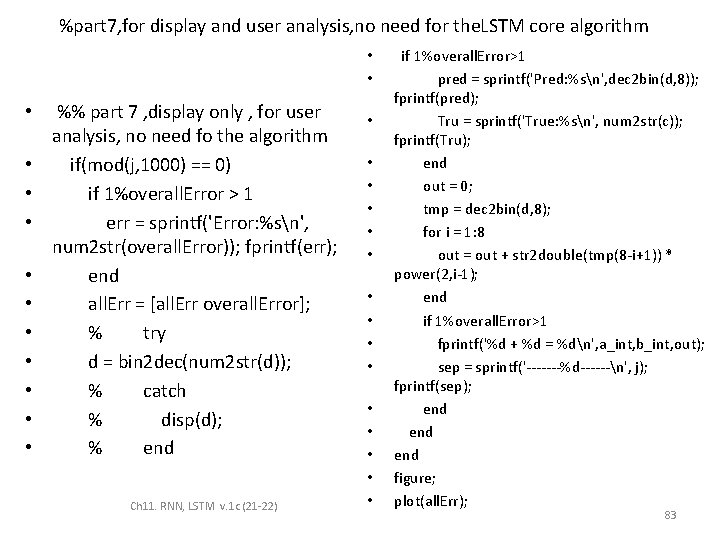
%part 7, for display and user analysis, no need for the. LSTM core algorithm • • • • %% part 7 , display only , for user analysis, no need fo the algorithm if(mod(j, 1000) == 0) if 1%overall. Error > 1 err = sprintf('Error: %sn', num 2 str(overall. Error)); fprintf(err); end all. Err = [all. Err overall. Error]; % try d = bin 2 dec(num 2 str(d)); % catch % disp(d); % end Ch 11. RNN, LSTM v. 1 c (21 -22) • • • • if 1%overall. Error>1 pred = sprintf('Pred: %sn', dec 2 bin(d, 8)); fprintf(pred); Tru = sprintf('True: %sn', num 2 str(c)); fprintf(Tru); end out = 0; tmp = dec 2 bin(d, 8); for i = 1: 8 out = out + str 2 double(tmp(8 -i+1)) * power(2, i-1); end if 1%overall. Error>1 fprintf('%d + %d = %dn', a_int, b_int, out); sep = sprintf('-------%d------n', j); fprintf(sep); end end figure; plot(all. Err); 83

• • • • • • • • • • • • • • • • • • • • • • • • • • • • • • • • • • • • • • • • • • • • • • • • • • • • • • • • • • • • • • • • • • • • • • • • • • • • • • • • • • • • • • • • • • • • %khwong 12 sept. 2017 %http: //blog. csdn. net/u 010866505/article/details/74910525 %http: //blog. sina. com. cn/s/blog_a 5 fdbf 010102 w 7 y 8. html %https: //iamtrask. github. io/2015/11/15/anyone-can-code-lstm/ %http: //blog. csdn. net/u 010866505/article/details/74910525 code % implementation of LSTM %function g=lstm_demo %-------LSTM-Matlab---------% implementation of LSTM %% part 1 , system setup function lstm_x() clc % clear close all %% training dataset generation binary_dim = 8; largest_number = 2^binary_dim - 1; binary = cell(largest_number, 1); for i = 1: largest_number + 1 binary{i} = dec 2 bin(i-1, binary_dim); int 2 binary{i} = binary{i}; end %% input variables alpha = 0. 1; input_dim = 2; hidden_dim = 32; output_dim = 1; all. Err = []; %% part 2 , initlize weight/variables %% initialize neural network weights % in_gate = sigmoid(X(t) * X_i + H(t-1) * H_i) ------- (1) X_i = 2 * rand(input_dim, hidden_dim) - 1; H_i = 2 * rand(hidden_dim, hidden_dim) - 1; X_i_update = zeros(size(X_i)); H_i_update = zeros(size(H_i)); bi = 2*rand(1, 1) - 1; bi_update = 0; % forget_gate = sigmoid(X(t) * X_f + H(t-1) * H_f) ------- (2) X_f = 2 * rand(input_dim, hidden_dim) - 1; H_f = 2 * rand(hidden_dim, hidden_dim) - 1; X_f_update = zeros(size(X_f)); H_f_update = zeros(size(H_f)); bf = 2*rand(1, 1) - 1; bf_update = 0; % out_gate = sigmoid(X(t) * X_o + H(t-1) * H_o) ------- (3) X_o = 2 * rand(input_dim, hidden_dim) - 1; H_o = 2 * rand(hidden_dim, hidden_dim) - 1; X_o_update = zeros(size(X_o)); H_o_update = zeros(size(H_o)); bo = 2*rand(1, 1) - 1; bo_update = 0; % g_gate = tanh(X(t) * X_g + H(t-1) * H_g) ------- (4) X_g = 2 * rand(input_dim, hidden_dim) - 1; H_g = 2 * rand(hidden_dim, hidden_dim) - 1; X_g_update = zeros(size(X_g)); H_g_update = zeros(size(H_g)); bg = 2*rand(1, 1) - 1; bg_update = 0; Code : LSTM_x 4 a. m out_para = 2 * rand(hidden_dim, output_dim) - 1; out_para_update = zeros(size(out_para)); % C(t) = C(t-1). * forget_gate + g_gate. * in_gate ------- (5) % S(t) = tanh(C(t)). * out_gate ------- (6) % Out = sigmoid(S(t) * out_para) ------- (7) % Note: Equations (1)-(6) are cores of LSTM in forward, and equation (7) is % used to transfer hiddent layer to predicted output, i. e. , the output layer. % (Sometimes you can use softmax for equation (7)) %% train, set iter=99999 by default %% part 3 a, main training loop, setup input/output for training. For each epcoh iter = 99999; %if =9999 iterations, shorter, faster, may not be accurate enough for j = 1: iter %% part 3 b % generate input/output a simple addition problem (a + b = c) a_int = randi(round(largest_number/2)); % int version a = int 2 binary{a_int+1}; % binary encoding b_int = randi(floor(largest_number/2)); % int version b = int 2 binary{b_int+1}; % binary encoding % true answer c_int = a_int + b_int; c = int 2 binary{c_int+1}; % int version % binary encoding % where we'll store our best guess (binary encoded) d = zeros(size(c)); if length(d)<8 pause; end % total error overall. Error = 0; % difference in output layer, i. e. , (target - out) output_deltas = []; % values of hidden layer, i. e. , S(t) hidden_layer_values = []; cell_gate_values = []; % initialize S(0) as a zero-vector hidden_layer_values = [hidden_layer_values; zeros(1, hidden_dim)]; cell_gate_values = [cell_gate_values; zeros(1, hidden_dim)]; % initialize memory gate % hidden layer H = []; H = [H; zeros(1, hidden_dim)]; % cell gate C = []; C = [C; zeros(1, hidden_dim)]; % in gate I = []; % forget gate F = []; % out gate O = []; % g gate G = []; %% part 4 , forward pass of training, for all 8 -bits % Forward pass: start to process a sequence, % Note: the output of a LSTM cell is the hidden_layer, and you need to % transfer it to predicted output for position = 0: binary_dim-1 %from bit 0 to highest bit % X ------> input, size: 1 x input_dim X = [a(binary_dim - position)-'0' b(binary_dim - position)-'0']; % y ------> label, size: 1 x output_dim y = [c(binary_dim - position)-'0']'; % use equations (1)-(7) in a forward pass. here we do not use bias in_gate = sigmoid(X * X_i + H(end, : ) * H_i + bi); % eq. (1) forget_gate = sigmoid(X * X_f + H(end, : ) * H_f + bf); % eq. (2) out_gate = sigmoid(X * X_o + H(end, : ) * H_o + bo); % eq. (3) g_gate = tan_h(X * X_g + H(end, : ) * H_g + bg); % eq. (4) C_t = C(end, : ). * forget_gate + g_gate. * in_gate; % eq. (5) H_t = tan_h(C_t). * out_gate; % eq. (6) % store these memory gates I = [I; in_gate]; F = [F; forget_gate]; O = [O; out_gate]; G = [G; g_gate]; C = [C; C_t]; H = [H; H_t]; % compute predict output pred_out = sigmoid(H_t * out_para); % compute error in output layer output_error = y - pred_out; % compute difference in output layer using derivative output_deltas = [output_deltas; output_error]; %*sigmoid_output_to_derivative(pred_out)]; % output_deltas = [output_deltas; output_error*(pred_out)]; % compute total error % note that if the size of pred_out or target is 1 x n or m x n, % you should use other approach to compute error. here the dimension % of pred_out is 1 x 1 overall. Error = overall. Error + abs(output_error(1)); % decode estimate so we can print it out d(binary_dim - position) = round(pred_out); end % from the last LSTM cell, you need a initial hidden layer difference future_H_diff = zeros(1, hidden_dim); %% part 5 , backward pass of training for all 8 -bits % back-propagation pass % the goal is to compute differences and use them to update weights % start from the last LSTM cell for position = 0: binary_dim-1 %from bit 0 to highest bit X = [a(position+1)-'0' b(position+1)-'0']; % hidden layer H_t = H(end-position, : ); % H(t) % previous hidden layer H_t_1 = H(end-position-1, : ); % H(t-1) C_t = C(end-position, : ); % C(t) C_t_1 = C(end-position-1, : ); % C(t-1) O_t = O(end-position, : ); F_t = F(end-position, : ); G_t = G(end-position, : ); I_t = I(end-position, : ); % output layer difference output_diff = output_deltas(end-position, : ); % hidden layer difference H_t_diff = output_diff * (out_para'); % out_para_diff = (H_t') * output_diff; % % out_gate diference O_t_diff = H_t_diff. *tan_h(C_t). *sigmoid_output_to_derivative(O_t); % C_t difference C_t_diff = H_t_diff. * O_t. * tan_h_output_to_derivative(C_t); % forget_gate_diffeence F_t_diff = C_t_diff. * C_t_1. * sigmoid_output_to_derivative(F_t); % in_gate difference I_t_diff = C_t_diff. * G_t. * sigmoid_output_to_derivative(I_t); % g_gate difference G_t_diff = C_t_diff. * I_t. * tan_h_output_to_derivative(G_t); % differences of X_i and H_i X_i_diff = X' * I_t_diff; % H_i_diff = (H_t_1)' * I_t_diff; % % differences of X_o and H_o X_o_diff = X' * O_t_diff; % H_o_diff = (H_t_1)' * O_t_diff; % % differences of X_o and H_o X_f_diff = X' * F_t_diff; % H_f_diff = (H_t_1)' * F_t_diff; % % differences of X_o and H_o X_g_diff = X' * G_t_diff; %. * tan_h_output_to_derivative(X_g); H_g_diff = (H_t_1)' * G_t_diff; %. * tan_h_output_to_derivative(H_g); % update X_i_update = X_i_update + X_i_diff; H_i_update = H_i_update + H_i_diff; X_o_update = X_o_update + X_o_diff; H_o_update = H_o_update + H_o_diff; X_f_update = X_f_update + X_f_diff; H_f_update = H_f_update + H_f_diff; X_g_update = X_g_update + X_g_diff; H_g_update = H_g_update + H_g_diff; bi_update = bi_update + I_t_diff; bo_update = bo_update + O_t_diff; bf_update = bf_update + F_t_diff; bg_update = bg_update + G_t_diff; out_para_update = out_para_update + out_para_diff; end %% part 6 , backward pass of training for all 8 -bits %Update all weights X_i = X_i + X_i_update * alpha; H_i = H_i + H_i_update * alpha; X_o = X_o + X_o_update * alpha; H_o = H_o + H_o_update * alpha; X_f = X_f + X_f_update * alpha; H_f = H_f + H_f_update * alpha; X_g = X_g + X_g_update * alpha; H_g = H_g + H_g_update * alpha; bi = bi + bi_update * alpha; bo = bo + bo_update * alpha; bf = bf + bf_update * alpha; bg = bg + bg_update * alpha; out_para = out_para + out_para_update * alpha; X_i_update = X_i_update * 0; H_i_update = H_i_update * 0; X_o_update = X_o_update * 0; H_o_update = H_o_update * 0; X_f_update = X_f_update * 0; H_f_update = H_f_update * 0; X_g_update = X_g_update * 0; H_g_update = H_g_update * 0; bi_update = 0; bf_update = 0; bo_update = 0; bg_update = 0; out_para_update = out_para_update * 0; %% part 7 , dispaly only , for user analysis, no need fo the algorithm if(mod(j, 1000) == 0) if 1%overall. Error > 1 err = sprintf('Error: %sn', num 2 str(overall. Error)); fprintf(err); end all. Err = [all. Err overall. Error]; % try d = bin 2 dec(num 2 str(d)); % catch % disp(d); % end if 1%overall. Error>1 pred = sprintf('Pred: %sn', dec 2 bin(d, 8)); fprintf(pred); Tru = sprintf('True: %sn', num 2 str(c)); fprintf(Tru); end out = 0; tmp = dec 2 bin(d, 8); for i = 1: 8 out = out + str 2 double(tmp(8 -i+1)) * power(2, i-1); end if 1%overall. Error>1 fprintf('%d + %d = %dn', a_int, b_int, out); sep = sprintf('-------%d------n', j); fprintf(sep); end end figure; plot(all. Err); %%%%%%%%%%%%%%%%%%%%%%%%%%%%%%%%%%%%%%%%%%%%%%%%%%%%%%%%%%%%%%%%%%%%%%%%%%% %part 8, testing , after weights are tranined, you machien can add 2 numbers for jj=1: 10 %randomly test 10 numbers % generate a simple addition problem (a + b = c) a_int = randi(round(largest_number/2)); % int version a = int 2 binary{a_int+1}; % binary encoding b_int = randi(floor(largest_number/2)); % int version b = int 2 binary{b_int+1}; % binary encoding % true answer c_int = a_int + b_int; c = int 2 binary{c_int+1}; % int version % binary encoding % where we'll store our best guess (binary encoded) d = zeros(size(c)); if length(d)<8 pause; end % total error overall. Error = 0; % difference in output layer, i. e. , (target - out) output_deltas = []; % values of hidden layer, i. e. , S(t) hidden_layer_values = []; cell_gate_values = []; % initialize S(0) as a zero-vector hidden_layer_values = [hidden_layer_values; zeros(1, hidden_dim)]; cell_gate_values = [cell_gate_values; zeros(1, hidden_dim)]; % initialize memory gate % hidden layer H = []; H = [H; zeros(1, hidden_dim)]; % cell gate C = []; C = [C; zeros(1, hidden_dim)]; % in gate I = []; % forget gate F = []; % out gate O = []; % g gate G = []; % start to process a sequence, i. e. , a forward pass % Note: the output of a LSTM cell is the hidden_layer, and you need to % transfer it to predicted output for position = 0: binary_dim-1 % X ------> input, size: 1 x input_dim X = [a(binary_dim - position)-'0' b(binary_dim - position)-'0']; Ch 11. RNN, LSTM v. 1 c (21 -22) 84

Student Exercise • 4 input neurons, 2 output neurons, 16 weights for each neuron. • How many weights and biases in the network? • Draw a data flow diagram of an LSTM with weights. Ch 11. RNN, LSTM v. 1 c (21 -22) 85

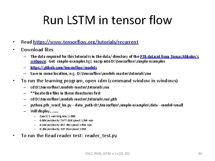
Run LSTM in tensor flow • • Read https: //www. tensorflow. org/tutorials/recurrent Download files – The data required for this tutorial is in the data/ directory of the PTB dataset from Tomas Mikolov's webpage. Get simple-examples. tgz, unzip into D: tensorflowsimple-examples – https: //github. com/tensorflow/models – Save in some location, e. g. D: tensorflowmodels-mastertutorialsrnn • To run the learning program, open cdm (command window in windows) – – – cd D: tensorflowmodels-mastertutorialsrnn **locate the files in these directories first cd D: tensorflowmodels-mastertutorialsrnnptb python ptb_word_lm. py --data_path=D: tensorflowsimple-examplesdata --model=small Will display, , …… • • • Epoch: 1 Learning rate: 1. 000 0. 004 perplexity: 7977. 018 speed: 1398 wps 0. 104 perplexity: 857. 681 speed: 1658 wps 0. 204 perplexity: 627. 014 speed: 1666 To run the Read reader test: reader_test. py Ch 11. RNN, LSTM v. 1 c (21 -22) 86

Extensions of LSTM • Gated Recurrent Unit (GRU) • CNN (convolution neural network)+LSTM (long short-term memory) Ch 11. RNN, LSTM v. 1 c (21 -22) 87

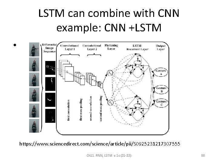
LSTM can combine with CNN example: CNN +LSTM • https: //www. sciencedirect. com/science/article/pii/S 0925231217307555 Ch 11. RNN, LSTM v. 1 c (21 -22) 88

Tensorflow example • https: //github. com/aymericdamien/Tensor. Flo w. Examples/blob/master/examples/3_Neural. Ne tworks/recurrent_network. py • LSTM for MNIST data optical character recognition Ch 11. RNN, LSTM v. 1 c (21 -22) 89

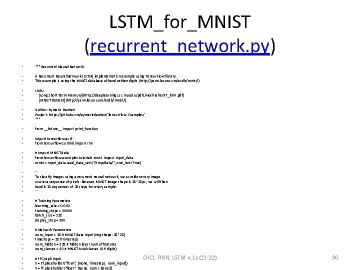
LSTM_for_MNIST (recurrent_network. py) • """ Recurrent Neural Network. • • A Recurrent Neural Network (LSTM) implementation example using Tensor. Flow library. This example is using the MNIST database of handwritten digits (http: //yann. lecun. com/exdb/mnist/) • • • Links: [Long Short Term Memory](http: //deeplearning. cs. cmu. edu/pdfs/Hochreiter 97_lstm. pdf) [MNIST Dataset](http: //yann. lecun. com/exdb/mnist/). • • • Author: Aymeric Damien Project: https: //github. com/aymericdamien/Tensor. Flow-Examples/ """ • from __future__ import print_function • • import tensorflow as tf from tensorflow. contrib import rnn • • • # Import MNIST data from tensorflow. examples. tutorials. mnist import input_data mnist = input_data. read_data_sets("/tmp/data/", one_hot=True) • • • ''' To classify images using a recurrent neural network, we consider every image row as a sequence of pixels. Because MNIST image shape is 28*28 px, we will then handle 28 sequences of 28 steps for every sample. ''' • • • # Training Parameters learning_rate = 0. 001 training_steps = 10000 batch_size = 128 display_step = 200 • • • # Network Parameters num_input = 28 # MNIST data input (img shape: 28*28) timesteps = 28 # timesteps num_hidden = 128 # hidden layer num of features num_classes = 10 # MNIST total classes (0 -9 digits) • • • # tf Graph input X = tf. placeholder("float", [None, timesteps, num_input]) Y = tf. placeholder("float", [None, num_classes]) Ch 11. RNN, LSTM v. 1 c (21 -22) 90

Summary • Introduced the idea of Recurrent Neural Networks RNN and Long Short-Term Memory LSTM • Gave and explained an example of implementing a digital adder of using LSTM Ch 11. RNN, LSTM v. 1 c (21 -22) 91

References • • • Deep Learning Book. http: //www. deeplearningbook. org/ • • Papers: Fully convolutional networks for semantic segmentation by J Long, Sequence to sequence learning with neural networks by tutorials http: //colah. github. io/posts/2015 -08 -Understanding-LSTMs/ https: //github. com/terryum/awesome-deep-learning-papers • • • turtorial: https: //theneuralperspective. com/tag/tutorials/ • • • RNN encoder-decoder https: //theneuralperspective. com/2016/11/20/recurrent-neural-networks-rnn-part-3 -encoder-decoder/ sequence to sequence model E Shelhamer, T Darrell I Sutskever, O Vinyals, QV Le - – – – https: //arxiv. org/pdf/1703. 01619. pdf https: //indico. io/blog/sequence-modeling-neuralnets-part 1/ https: //medium. com/towards-data-science/lstm-by-example-using-tensorflow-feb 0 c 1968537 https: //google. github. io/seq 2 seq/nmt/ https: //chunml. github. io/Chun. ML. github. io/project/Sequence-To-Sequence/ parameters of lstm • • https: //stackoverflow. com/questions/38080035/how-to-calculate-the-number-of-parameters-of-an-lstm-network https: //datascience. stackexchange. com/questions/10615/number-of-parameters-in-an-lstm-model https: //stackoverflow. com/questions/38080035/how-to-calculate-the-number-of-parameters-of-an-lstm-network https: //www. quora. com/What-is-the-meaning-of-%E 2%80%9 CThe-number-of-units-in-the-LSTM-cell https: //www. quora. com/In-LSTM-how-do-you-figure-out-what-size-the-weights-are-supposed-to-be http: //kbullaughey. github. io/lstm-play/lstm/ (batch size example) – feedback – Numerical examples • • https: //medium. com/@aidangomez/let-s-do-this-f 9 b 699 de 31 d 9 https: //blog. aidangomez. ca/2016/04/17/Backpropogating-an-LSTM-A-Numerical-Example/ https: //karanalytics. wordpress. com/2017/06/06/sequence-modelling-using-deep-learning/ http: //monik. in/a-noobs-guide-to-implementing-rnn-lstm-using-tensorflow/ Ch 11. RNN, LSTM v. 1 c (21 -22) 92

Appendix Ch 11. RNN, LSTM v. 1 c (21 -22) 93

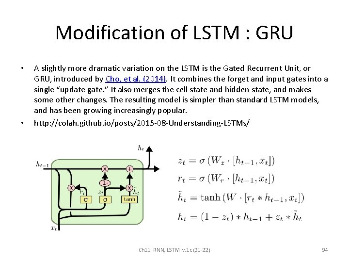
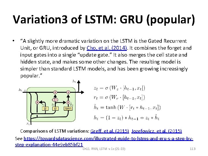
Modification of LSTM : GRU • • A slightly more dramatic variation on the LSTM is the Gated Recurrent Unit, or GRU, introduced by Cho, et al. (2014). It combines the forget and input gates into a single “update gate. ” It also merges the cell state and hidden state, and makes some other changes. The resulting model is simpler than standard LSTM models, and has been growing increasingly popular. http: //colah. github. io/posts/2015 -08 -Understanding-LSTMs/ Ch 11. RNN, LSTM v. 1 c (21 -22) 94

Appendix 1 a: Using Square error for output measurement Ch 11. RNN, LSTM v. 1 c (21 -22) 95

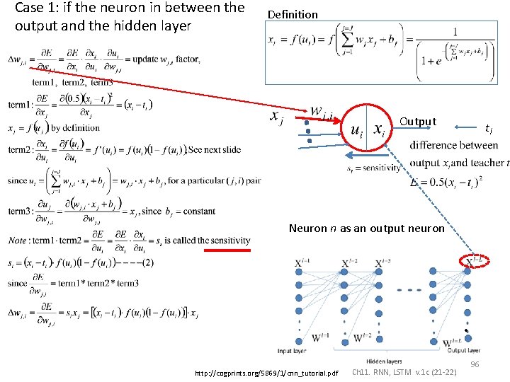
Case 1: if the neuron in between the output and the hidden layer Definition Output ti Neuron n as an output neuron • http: //cogprints. org/5869/1/cnn_tutorial. pdf Ch 11. RNN, LSTM v. 1 c (21 -22) 96

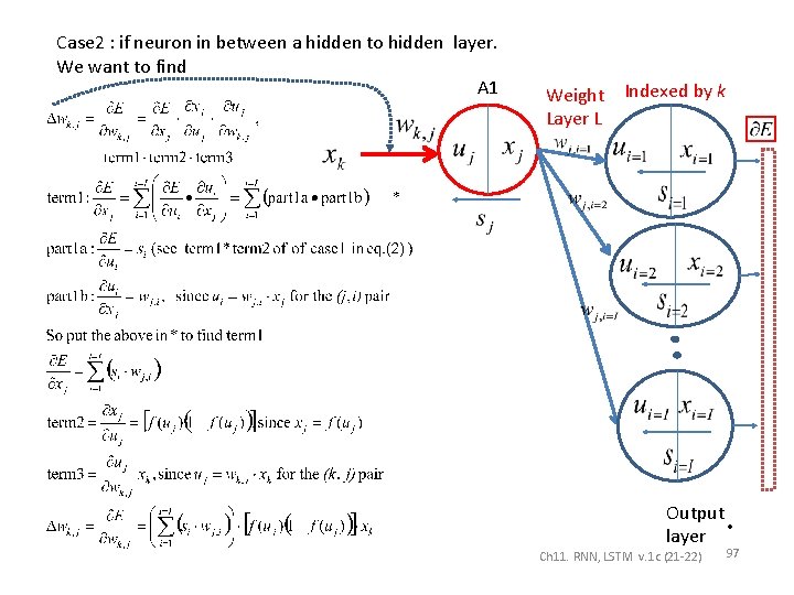
Case 2 : if neuron in between a hidden to hidden layer. We want to find A 1 Weight Layer L Indexed by k Output layer • Ch 11. RNN, LSTM v. 1 c (21 -22) 97

Appendix 1 b Using softmax with cross-entropy_loss for a 2 -classifier (single output neuron) Ch 11. RNN, LSTM v. 1 c (21 -22) 98

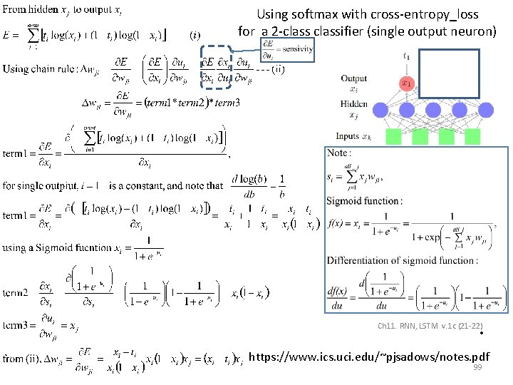
Using softmax with cross-entropy_loss for a 2 -classifier (single output neuron) Ch 11. RNN, LSTM v. 1 c (21 -22) • https: //www. ics. uci. edu/~pjsadows/notes. pdf 99

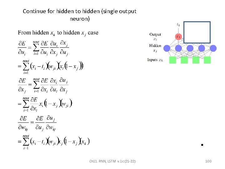
Continue for hidden to hidden (single output neuron) • Ch 11. RNN, LSTM v. 1 c (21 -22) 100

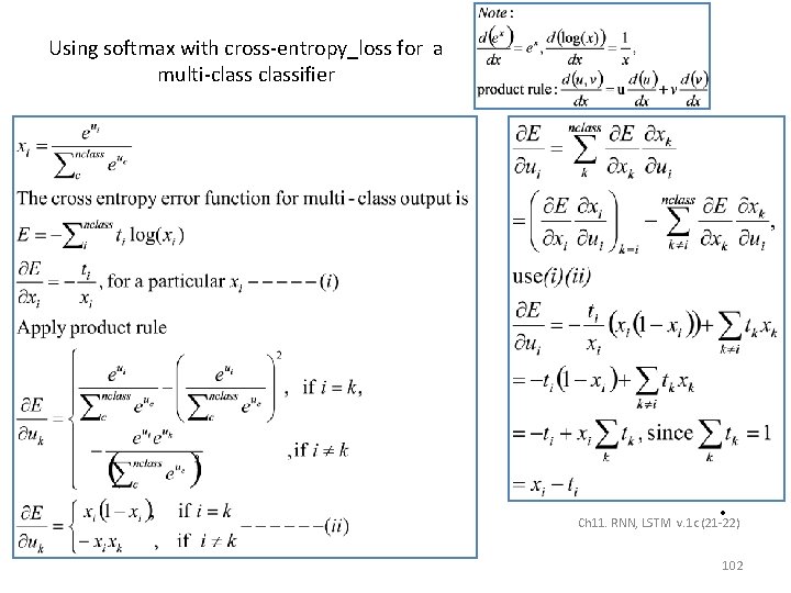
Appendix 1 c Using softmax with crossentropy_loss for a mult-classifier https: //www. ics. uci. edu/~pjsadows/notes. pdf Ch 11. RNN, LSTM v. 1 c (21 -22) 101

Using softmax with cross-entropy_loss for a multi-classifier • Ch 11. RNN, LSTM v. 1 c (21 -22) 102

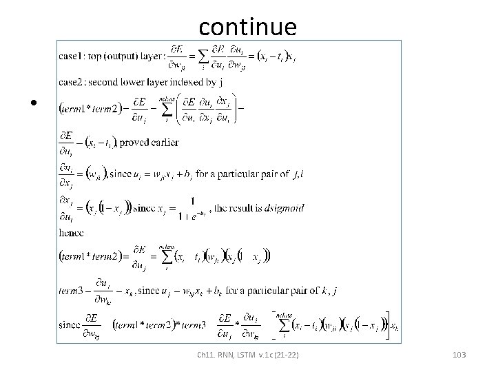
continue • Ch 11. RNN, LSTM v. 1 c (21 -22) 103

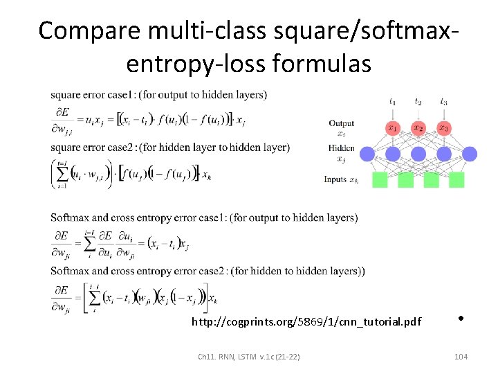
Compare multi-class square/softmaxentropy-loss formulas http: //cogprints. org/5869/1/cnn_tutorial. pdf Ch 11. RNN, LSTM v. 1 c (21 -22) • 104

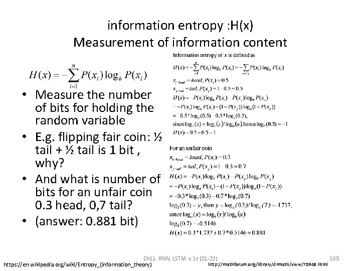
information entropy : H(x) Measurement of information content • Measure the number of bits for holding the random variable • E. g. flipping fair coin: ½ tail + ½ tail is 1 bit , why? • And what is number of bits for an unfair coin 0. 3 head, 0, 7 tail? • (answer: 0. 881 bit) Ch 11. RNN, LSTM v. 1 c (21 -22) 105 http: //mathforum. org/library/drmath/view/70648. html https: //en. wikipedia. org/wiki/Entropy_(information_theory)

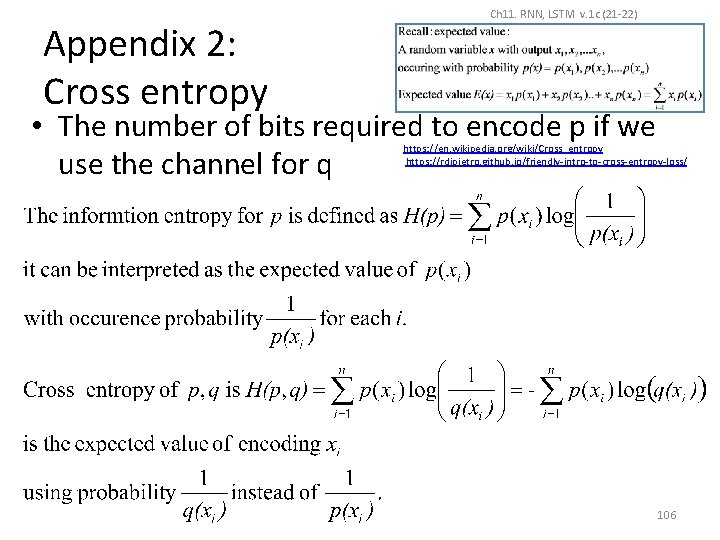
Appendix 2: Cross entropy Ch 11. RNN, LSTM v. 1 c (21 -22) • The number of bits required to encode p if we use the channel for q https: //en. wikipedia. org/wiki/Cross_entropy https: //rdipietro. github. io/friendly-intro-to-cross-entropy-loss/ 106

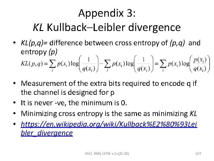
Appendix 3: KL Kullback–Leibler divergence • KL(p, q)= difference between cross entropy of (p, q) and entropy (p) • Measurement of the extra bits required to encode q if the channel is designed for p • It is never -ve, the minimum is 0. • Minimizing cross entropy is the same as minimizing KL • https: //en. wikipedia. org/wiki/Kullback%E 2%80%93 Lei bler_divergence Ch 11. RNN, LSTM v. 1 c (21 -22) 107

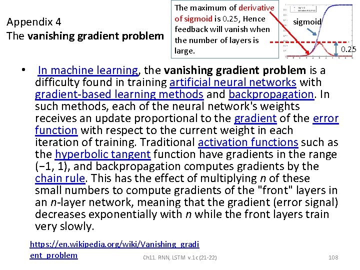
Appendix 4 The vanishing gradient problem The maximum of derivative of sigmoid is 0. 25, Hence feedback will vanish when the number of layers is large. sigmoid 0. 25 • In machine learning, the vanishing gradient problem is a difficulty found in training artificial neural networks with gradient-based learning methods and backpropagation. In such methods, each of the neural network's weights receives an update proportional to the gradient of the error function with respect to the current weight in each iteration of training. Traditional activation functions such as the hyperbolic tangent function have gradients in the range (− 1, 1), and backpropagation computes gradients by the chain rule. This has the effect of multiplying n of these small numbers to compute gradients of the "front" layers in an n-layer network, meaning that the gradient (error signal) decreases exponentially with n while the front layers train very slowly. https: //en. wikipedia. org/wiki/Vanishing_gradi ent_problem Ch 11. RNN, LSTM v. 1 c (21 -22) 108

Solutions to the vanishing gradient problem • Multi-level hierarchy – • Related approach – • To overcome this problem, several methods were proposed. One is Jürgen Schmidhuber's multi-level hierarchy of networks (1992) pre-trained one level at a time through unsupervised learning, fine-tuned through backpropagation. [3] Here each level learns a compressed representation of the observations that is fed to the next level. Similar ideas have been used in feed-forward neural network for unsupervised pre-training to structure a neural network, making it first learn generally useful feature detectors. Then the network is trained further by supervised back-propagation to classify labeled data. The Deep belief network model by Hinton et al. (2006) involves learning the distribution of a high level representation using successive layers of binary or real-valued latent variables. It uses a restricted Boltzmann machine to model each new layer of higher level features. Each new layer guarantees an increase on the lower-bound of the log likelihood of the data, thus improving the model, if trained properly. Once sufficiently many layers have been learned the deep architecture may be used as a generative model by reproducing the data when sampling down the model (an "ancestral pass") from the top level feature activations. [4] Hinton reports that his models are effective feature extractors over high-dimensional, structured data. [5] This work plays a keyrole in reintroducing the interests in deep neural network research and consequently leads to the developments of Deep learning, although deep belief network is no longer the main deep learning technique. Long short-term memory – Another method particularly used for Recurrent neural network is the long short-term memory (LSTM) network of 1997 by Hochreiter & Schmidhuber. [6] In 2009, deep multidimensional LSTM networks demonstrated the power of deep learning with many nonlinear layers, by winning three ICDAR 2009 competitions in connected handwriting recognition, without any prior knowledge about the three different languages to be learned. [7][8] Ch 11. RNN, LSTM v. 1 c (21 -22) 109

Variations of LSTM Alternative implementations Ch 11. RNN, LSTM v. 1 c (21 -22) 110

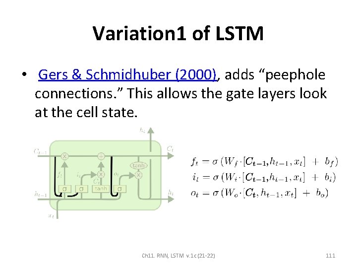
Variation 1 of LSTM • Gers & Schmidhuber (2000), adds “peephole connections. ” This allows the gate layers look at the cell state. Ch 11. RNN, LSTM v. 1 c (21 -22) 111

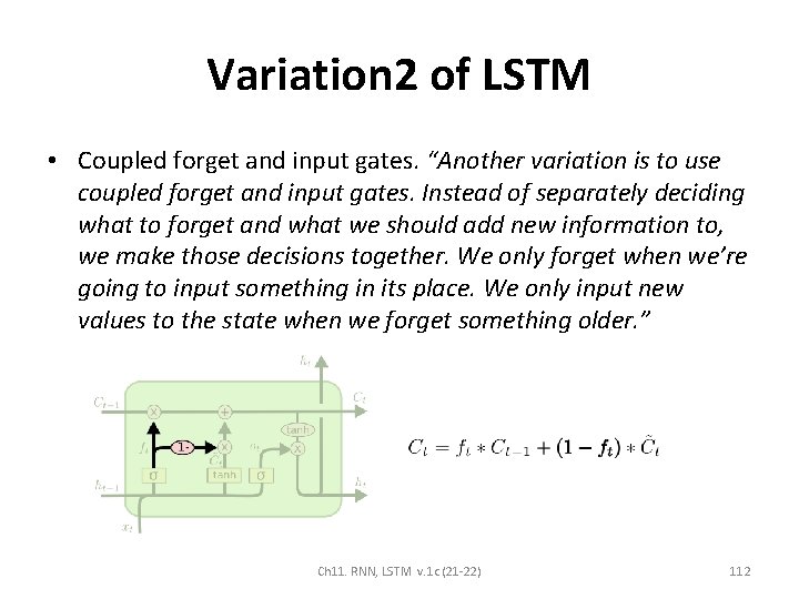
Variation 2 of LSTM • Coupled forget and input gates. “Another variation is to use coupled forget and input gates. Instead of separately deciding what to forget and what we should add new information to, we make those decisions together. We only forget when we’re going to input something in its place. We only input new values to the state when we forget something older. ” Ch 11. RNN, LSTM v. 1 c (21 -22) 112

Variation 3 of LSTM: GRU (popular) • “A slightly more dramatic variation on the LSTM is the Gated Recurrent Unit, or GRU, introduced by Cho, et al. (2014). It combines the forget and input gates into a single “update gate. ” It also merges the cell state and hidden state, and makes some other changes. The resulting model is simpler than standard LSTM models, and has been growing increasingly popular. ” Comparisons of LSTM variations: Greff, et al. (2015) Jozefowicz, et al. (2015) See https: //towardsdatascience. com/illustrated-guide-to-lstms-and-gru-s-a-step-bystep-explanation-44 e 9 eb 85 bf 21 Ch 11. RNN, LSTM v. 1 c (21 -22) 113

Solutions to the vanishing gradient problem • Multi-level hierarchy – • Related approach – • Similar ideas have been used in feed-forward neural network for unsupervised pre-training to structure a neural network, making it first learn generally useful feature detectors. Then the network is trained further by supervised back-propagation to classify labeled data. The Deep belief network model by Hinton et al. (2006) involves learning the distribution of a high level representation using successive layers of binary or real-valued latent variables. It uses a restricted Boltzmann machine to model each new layer of higher level features. Each new layer guarantees an increase on the lower-bound of the log likelihood of the data, thus improving the model, if trained properly. Once sufficiently many layers have been learned the deep architecture may be used as a generative model by reproducing the data when sampling down the model (an "ancestral pass") from the top level feature activations. [4] Hinton reports that his models are effective feature extractors over high-dimensional, structured data. [5] This work plays a keyrole in reintroducing the interests in deep neural network research and consequently leads to the developments of Deep learning, although deep belief network is no longer the main deep learning technique. Long short-term memory – • To overcome this problem, several methods were proposed. One is Jürgen Schmidhuber's multi-level hierarchy of networks (1992) pre-trained one level at a time through unsupervised learning, fine-tuned through backpropagation. [3] Here each level learns a compressed representation of the observations that is fed to the next level. Another method particularly used for Recurrent neural network is the long short-term memory (LSTM) network of 1997 by Hochreiter & Schmidhuber. [6] In 2009, deep multidimensional LSTM networks demonstrated the power of deep learning with many nonlinear layers, by winning three ICDAR 2009 competitions in connected handwriting recognition, without any prior knowledge about the three different languages to be learned. [7][8] GRU (Gated Recurrent Unit) Ch 11. RNN, LSTM v. 1 c (21 -22) 114

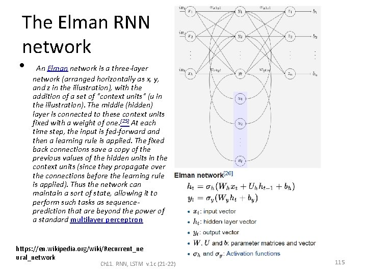
The Elman RNN network • An Elman network is a three-layer network (arranged horizontally as x, y, and z in the illustration), with the addition of a set of "context units" (u in the illustration). The middle (hidden) layer is connected to these context units fixed with a weight of one. [25] At each time step, the input is fed-forward and then a learning rule is applied. The fixed back connections save a copy of the previous values of the hidden units in the context units (since they propagate over the connections before the learning rule is applied). Thus the network can maintain a sort of state, allowing it to perform such tasks as sequenceprediction that are beyond the power of a standard multilayer perceptron https: //en. wikipedia. org/wiki/Recurrent_ne ural_network Ch 11. RNN, LSTM v. 1 c (21 -22) 115