Introduction to RNN Recurrent neural network KH Wong

Introduction to RNN (Recurrent neural network) KH Wong RNN & LSTM (g. 2. a) 1

Overview • • • Introduction Concept of RNN (Recurrent neural network) ? The Gradient vanishing problem LSTM theory and concept LSTM Numerical example RNN & LSTM (g. 2. a) 2

Introduction • RNN (Recurrent neural network) is a form of neural networks that feed outputs back to the inputs during operation • LSTM (Long short-term memory) is a form of RNN. It fixes the vanishing gradient problem of the original RNN. – Application: Sequence to sequence model based using LSTM for machine translation • • • References: Materials are mainly based on links found in https: //www. tensorflow. org/tutorials https: //towardsdatascience. com/illustrated-guide-to-lstms-and-gru-s-a-step-by-step-explanation 44 e 9 eb 85 bf 21 RNN & LSTM (g. 2. a) 3

Concept of RNN (Recurrent neural network) concept RNN & LSTM (g. 2. a) 4

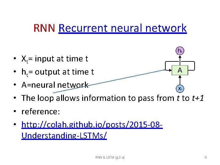
RNN Recurrent neural network • • • Xt= input at time t ht= output at time t A=neural network The loop allows information to pass from t to t+1 reference: http: //colah. github. io/posts/2015 -08 Understanding-LSTMs/ RNN & LSTM (g. 2. a) 5

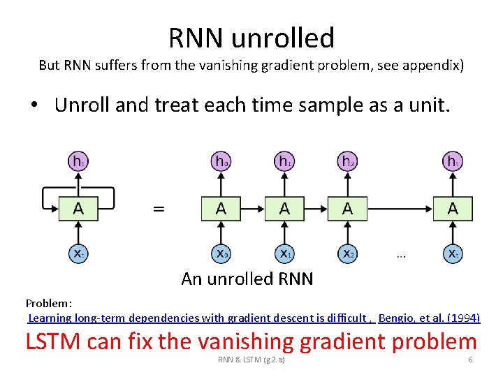
RNN unrolled But RNN suffers from the vanishing gradient problem, see appendix) • Unroll and treat each time sample as a unit. An unrolled RNN Problem: Learning long-term dependencies with gradient descent is difficult , Bengio, et al. (1994) LSTM can fix the vanishing gradient problem RNN & LSTM (g. 2. a) 6

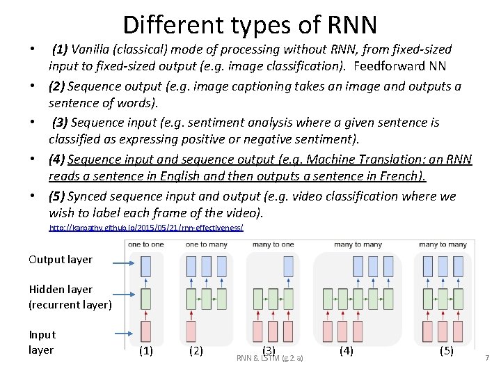
• • • Different types of RNN (1) Vanilla (classical) mode of processing without RNN, from fixed-sized input to fixed-sized output (e. g. image classification). Feedforward NN (2) Sequence output (e. g. image captioning takes an image and outputs a sentence of words). (3) Sequence input (e. g. sentiment analysis where a given sentence is classified as expressing positive or negative sentiment). (4) Sequence input and sequence output (e. g. Machine Translation: an RNN reads a sentence in English and then outputs a sentence in French). (5) Synced sequence input and output (e. g. video classification where we wish to label each frame of the video). http: //karpathy. github. io/2015/05/21/rnn-effectiveness/ Output layer Hidden layer (recurrent layer) Input layer (1) (2) (3) RNN & LSTM (g. 2. a) (4) (5) 7

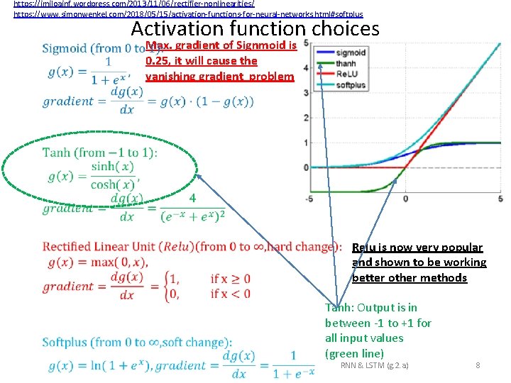
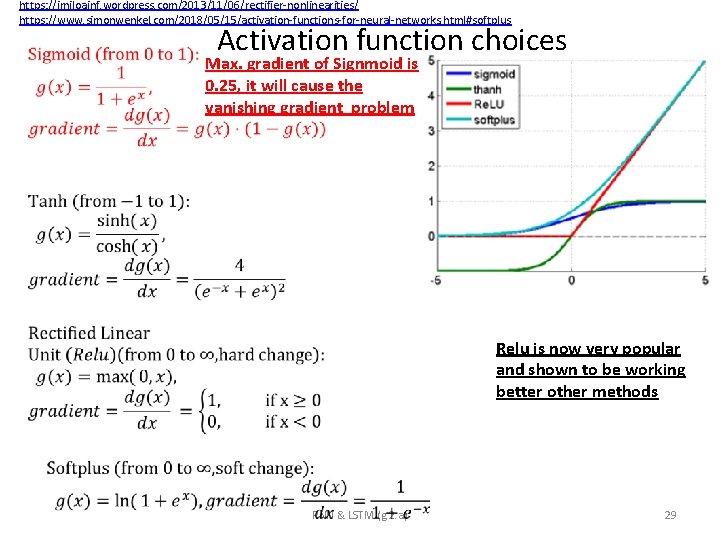
https: //imiloainf. wordpress. com/2013/11/06/rectifier-nonlinearities/ https: //www. simonwenkel. com/2018/05/15/activation-functions-for-neural-networks. html#softplus Activation function choices Max. gradient of Signmoid is 0. 25, it will cause the vanishing gradient problem Relu is now very popular and shown to be working better other methods Tanh: Output is in between -1 to +1 for all input values (green line) RNN & LSTM (g. 2. a) 8

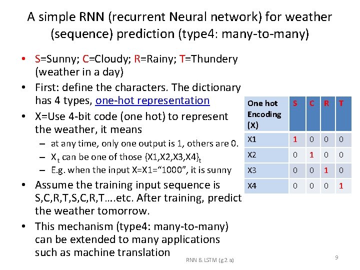
A simple RNN (recurrent Neural network) for weather (sequence) prediction (type 4: many-to-many) • S=Sunny; C=Cloudy; R=Rainy; T=Thundery (weather in a day) • First: define the characters. The dictionary has 4 types, one-hot representation • X=Use 4 -bit code (one hot) to represent the weather, it means One hot Encoding (X) – at any time, only one output is 1, others are 0. X 1 X 2 – X t can be one of those {X 1, X 2, X 3, X 4}t – E. g. when the input X=X 1=“ 1000”, it is sunny X 3 • Assume the training input sequence is S, C, R, T, S, C, R, T…. etc. After training, predict the weather tomorrow. • This mechanism (type 4: many-to-many) can be extended to many applications such as machine translation RNN & LSTM (g. 2. a) X 4 S C R T 1 0 0 0 0 1 9

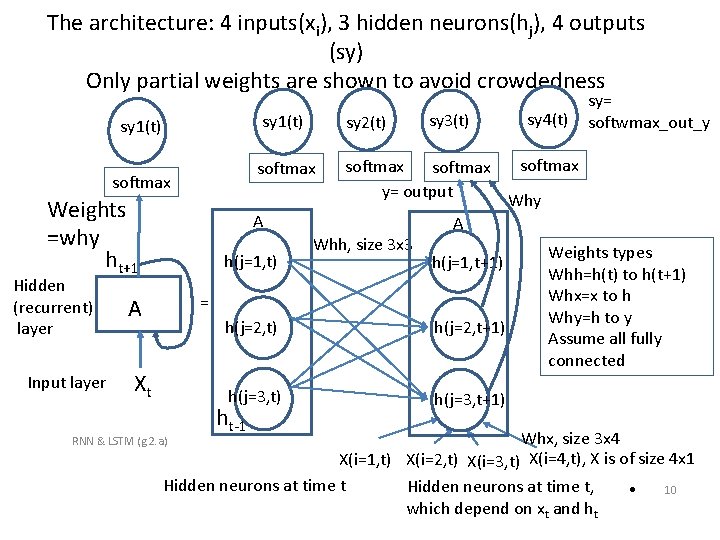
The architecture: 4 inputs(xi), 3 hidden neurons(hj), 4 outputs (sy) Only partial weights are shown to avoid crowdedness sy 1(t) softmax Weights =why ht+1 Hidden (recurrent) layer Input layer sy 2(t) softmax y= output A h(j=1, t) sy 3(t) Whh, size 3 x 3 Xt h(j=1, t+1) h(j=2, t+1) h(j=3, t+1) ht-1 softmax Why A = A sy 4(t) sy= softwmax_out_y Weights types Whh=h(t) to h(t+1) Whx=x to h Why=h to y Assume all fully connected Whx, size 3 x 4 X(i=1, t) X(i=2, t) X(i=3, t) X(i=4, t), X is of size 4 x 1 Hidden neurons at time t, • 10 which depend on xt and ht RNN & LSTM (g. 2. a)

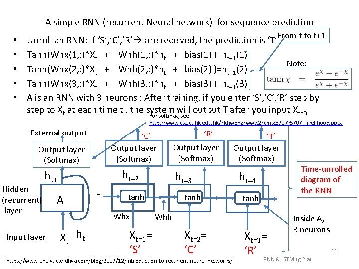
A simple RNN (recurrent Neural network) for sequence prediction • • • Unroll an RNN: If ‘S’, ’C’, ’R’ are received, the prediction is ‘T’From t to t+1 Tanh(Whx(1, : )*Xt + Whh(1, : )*ht + bias(1) )=ht+1(1) Note: Tanh(Whx(2, : )*Xt + Whh(2, : )*ht + bias(2) )=ht+1(2) Tanh(Whx(3, : )*Xt + Whh(3, : )*ht + bias(3) )=ht+1(3) A is an RNN with 3 neurons : After training, if you enter ‘S’, ’C’, ’R’ step by step to Xt at each time t , the system will output T after you input Xt=3 For softmax, see http: //www. cse. cuhk. edu. hk/~khwong/www 2/cmsc 5707/5707_likelihood. pptx External output ‘C’ Output layer (Softmax) Hidden (recurrent) layer ht=2 ht+1 Input layer A = Xt h t Xt=1= ‘S’ Output layer (Softmax) ht=3 tanh Whx ‘R’ tanh ‘T’ Output layer (Softmax) ht=4 tanh Whh Xt=2= ‘C’ https: //www. analyticsvidhya. com/blog/2017/12/introduction-to-recurrent-neural-networks/ Xt=3= ‘R’ Time-unrolled diagram of the RNN Inside A, 3 neurons RNN & LSTM (g. 2. a) 11

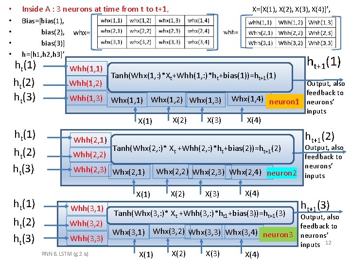
• Inside A : 3 neurons at time from t to t+1, • • Bias=[bias(1), bias(2), bias(3)] h=[h 1, h 2, h 3]’ ht(1) ht(2) ht(3) Whh(1, 1) Whh(1, 2) Tanh(Whx(1, : )*Xt+Whh(1, : )*ht+bias(1))=ht+1(1) Whh(1, 3) Whx(1, 1) Whx(1, 2) Whx(1, 3) X(1) ht(2) ht(3) ht(1) ht(2) ht(3) X=[X(1), X(2), X(3), X(4)]’, Whh(2, 1) Whh(2, 2) X(1) Whh(3, 2) Whh(3, 3) RNN & LSTM (g. 2. a) X(3) Output, also feedback to Whx(1, 4) neuron 1 neurons’ inputs X(4) Tanh(Whx(2, : )* Xt +Whh(2, : )*ht+bias(2))=ht+1(2) Whh(2, 3) Whx(2, 1) Whh(3, 1) X(2) Whx(2, 3) Whx(2, 4) neuron 2 X(2) X(3) ht+1(1) X(4) Tanh(Whx(3, : )* Xt +Whh(3, : )*ht 1+bias(3))=ht+1(3) ht+1(2) Output, also feedback to neurons’ inputs ht+1(3) Output, also feedback to Whx(3, 1) Whx(3, 2) Whx(3, 3) Whx(3, 4) neuron 3 neurons’ inputs 12 X(1) X(2) X(3) X(4)

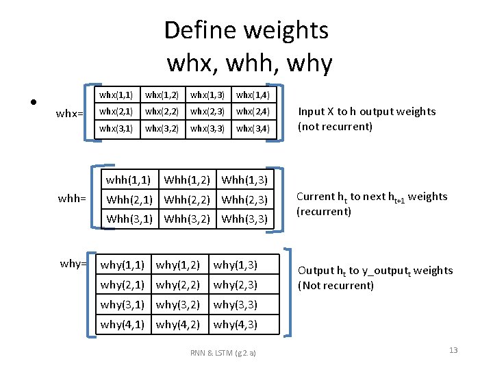
Define weights whx, whh, why • whx= whx(1, 1) whx(1, 2) whx(1, 3) whx(1, 4) whx(2, 1) whx(2, 2) whx(2, 3) whx(2, 4) whx(3, 1) whx(3, 2) whx(3, 3) whx(3, 4) whh(1, 1) whh= Whh(1, 2) Whh(1, 3) Whh(2, 1) Whh(2, 2) Whh(2, 3) Whh(3, 1) Whh(3, 2) Whh(3, 3) why= Input X to h output weights (not recurrent) why(1, 1) why(1, 2) why(1, 3) why(2, 1) why(2, 2) why(2, 3) why(3, 1) why(3, 2) why(3, 3) why(4, 1) why(4, 2) why(4, 3) RNN & LSTM (g. 2. a) Current ht to next ht+1 weights (recurrent) Output ht to y_outputt weights (Not recurrent) 13

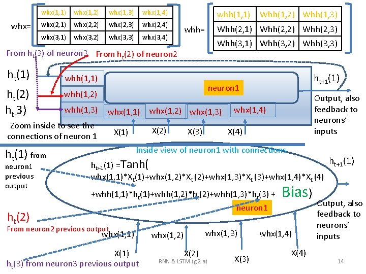
whx= whx(1, 1) whx(1, 2) whx(1, 3) whx(1, 4) whx(2, 1) whx(2, 2) whx(2, 3) whx(2, 4) whx(3, 1) whx(3, 2) whx(3, 3) whx(3, 4) whh(1, 1) Whh(2, 2) Whh(2, 3) whh= Whh(3, 1) Whh(3, 2) Whh(3, 3) From ht(3) of neuron 3 From ht(2) of neuron 2 ht(1) ht(2) ht-3) whh(1, 1) whx(1, 1) Zoom inside to see the connections of neuron 1 ht(1) from neuron 1 previous output ht(2) ht+1(1) neuron 1 whh(1, 2) whh(1, 3) Whh(1, 2) Whh(1, 3) whx(1, 2) whx(1, 3) X(2) X(1) Output, also feedback to neurons’ inputs whx(1, 4) X(3) Inside view of neuron 1 with connections ht+1(1) =Tanh( whx(1, 1)*Xt(1)+whx(1, 2)*Xt (2)+whx(1, 3)*Xt (3)+whx(1, 4)*Xt (4) +whh(1, 1)*ht(1)+whh(1, 2)*ht(2)+whh(1, 3)*ht(3) + neuron 1 From neuron 2 previous output whx(1, 1) X(1) ht(3) from neuron 3 previous output whx(1, 3) whx(1, 2) X(2) RNN & LSTM (g. 2. a) X(3) Bias) whx(1, 4) X(4) Output, also feedback to neurons’ inputs 14

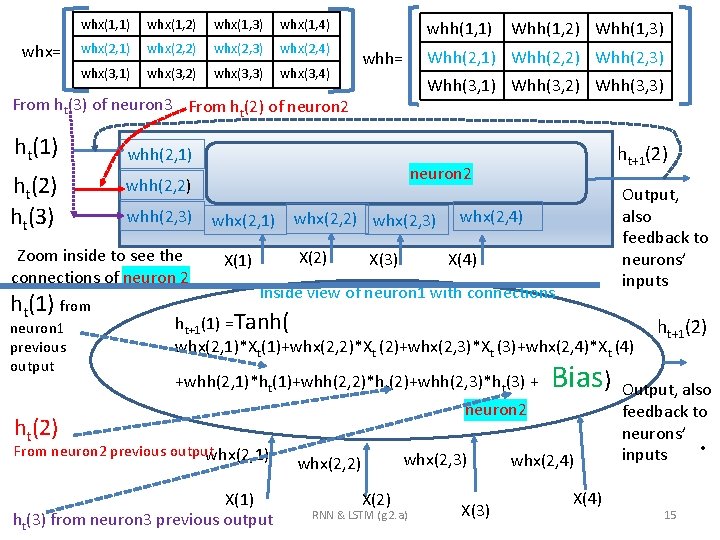
whx= whx(1, 1) whx(1, 2) whx(1, 3) whx(1, 4) whx(2, 1) whx(2, 2) whx(2, 3) whx(2, 4) whx(3, 1) whx(3, 2) whx(3, 3) whx(3, 4) whh(1, 1) Whh(2, 2) Whh(2, 3) whh= Whh(3, 1) Whh(3, 2) Whh(3, 3) From ht(3) of neuron 3 From ht(2) of neuron 2 ht(1) ht(2) ht(3) whh(2, 1) Zoom inside to see the connections of neuron 2 ht(1) from neuron 1 previous output ht+1(2) neuron 2 whh(2, 2) whh(2, 3) Whh(1, 2) Whh(1, 3) whx(2, 1) whx(2, 2) whx(2, 3) X(2) X(1) Output, also feedback to neurons’ inputs whx(2, 4) X(3) Inside view of neuron 1 with connections ht+1(1) =Tanh( whx(2, 1)*Xt(1)+whx(2, 2)*Xt (2)+whx(2, 3)*Xt (3)+whx(2, 4)*Xt (4) +whh(2, 1)*ht(1)+whh(2, 2)*ht(2)+whh(2, 3)*ht(3) + neuron 2 ht(2) From neuron 2 previous output whx(2, 1) X(1) ht(3) from neuron 3 previous output Bias) whx(2, 3) whx(2, 2) X(2) RNN & LSTM (g. 2. a) X(3) whx(2, 4) X(4) ht+1(2) Output, also feedback to neurons’ • inputs 15

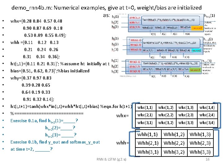
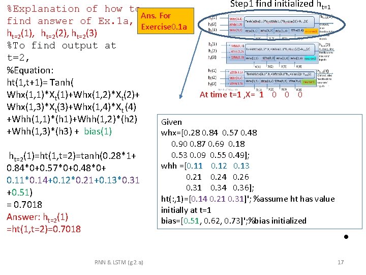
• • • • • demo_rnn 4 b. m: Numerical examples, give at t=0, weight/bias are initialized as: whx=[0. 28 0. 84 0. 57 0. 48 0. 90 0. 87 0. 69 0. 18 0. 53 0. 09 0. 55 0. 49]; whh =[0. 11 0. 12 0. 13 0. 21 0. 24 0. 26 0. 31 0. 34 0. 36]; ht(: , 1)=[0. 11 0. 21 0. 31]'; %assume ht initially at t=1 bias=[0. 51, 0. 62, 0. 73]'; %bias initialized why=[0. 37 0. 97 0. 83 0. 39 0. 28 0. 65 0. 64 0. 19 0. 33 0. 91 0. 32 0. 14]; ht(: , t+1)=tanh(whx*in(: , t)+whh*ht(: , t)+bias) %eqn. for h(t+1) %============== whx= Exercise 0. 1 a, find ht=2(1)=_____? ht=2(2)=_____? ht=2(3)= _____? Exercise 0. 1 b, find y_out and softmax_y_out whh= at time t=2, ______? RNN & LSTM (g. 2. a) whx(1, 1) whx(1, 2) whx(1, 3) whx(1, 4) whx(2, 1) whx(2, 2) whx(2, 3) whx(2, 4) whx(3, 1) whx(3, 2) whx(3, 3) whx(3, 4) whh(1, 1) Whh(1, 2) Whh(1, 3) Whh(2, 1) Whh(2, 2) Whh(2, 3) Whh(3, 1) Whh(3, 2) Whh(3, 3) 16

Step 1 find initialized ht=1 %Explanation of how to Ans. For find answer of Ex. 1 a, Exercise 0. 1 a ht=2(1), ht=2(2), ht=2(3) %To find output at t=2, %Equation: ht(1, t+1)= Tanh( At time t=1 , X= 1 0 0 0 Whx(1, 1)*Xt(1)+Whx(1, 2)*Xt(2)+ Whx(1, 3)*Xt(3)+Whx(1, 4)*Xt (4) +Whh(1, 1)*(h 1)+Whh(1, 2)*(h 2) Given +Whh(1, 3)*(h 3) + bias(1) whx=[0. 28 0. 84 0. 57 0. 48 ht=2(1)=ht(1, t=2)=tanh(0. 28*1+ 0. 84*0+0. 57*0+0. 48*0+ 0. 11*0. 14+0. 12*0. 21+0. 13*0. 31 +0. 51) = 0. 7018 Answer: ht=2(1) =ht(1, t=2)=0. 7018 RNN & LSTM (g. 2. a) 0. 90 0. 87 0. 69 0. 18 0. 53 0. 09 0. 55 0. 49]; whh =[0. 11 0. 12 0. 13 0. 21 0. 24 0. 26 0. 31 0. 34 0. 36]; ht(: , 1)=[0. 14 0. 21 0. 31]'; %assume ht has value initially at t=1 bias=[0. 51, 0. 62, 0. 73]'; %bias initialized • 17

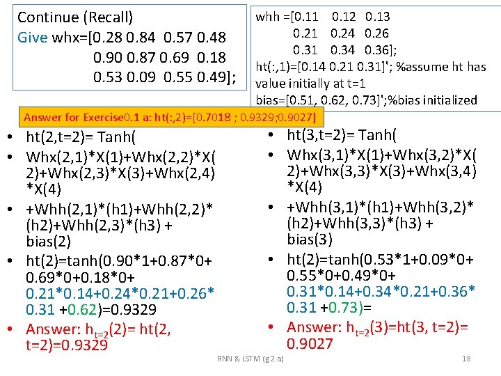
Continue (Recall) Give whx=[0. 28 0. 84 0. 57 0. 48 0. 90 0. 87 0. 69 0. 18 0. 53 0. 09 0. 55 0. 49]; whh =[0. 11 0. 12 0. 13 0. 21 0. 24 0. 26 0. 31 0. 34 0. 36]; ht(: , 1)=[0. 14 0. 21 0. 31]'; %assume ht has value initially at t=1 bias=[0. 51, 0. 62, 0. 73]'; %bias initialized Answer for Exercise 0. 1 a: ht(: , 2)=[0. 7018 ; 0. 9329; 0. 9027] • ht(2, t=2)= Tanh( • Whx(2, 1)*X(1)+Whx(2, 2)*X( 2)+Whx(2, 3)*X(3)+Whx(2, 4) *X(4) • +Whh(2, 1)*(h 1)+Whh(2, 2)* (h 2)+Whh(2, 3)*(h 3) + bias(2) • ht(2)=tanh(0. 90*1+0. 87*0+ 0. 69*0+0. 18*0+ 0. 21*0. 14+0. 24*0. 21+0. 26* 0. 31 +0. 62)=0. 9329 • Answer: ht=2(2)= ht(2, t=2)=0. 9329 • ht(3, t=2)= Tanh( • Whx(3, 1)*X(1)+Whx(3, 2)*X( 2)+Whx(3, 3)*X(3)+Whx(3, 4) *X(4) • +Whh(3, 1)*(h 1)+Whh(3, 2)* (h 2)+Whh(3, 3)*(h 3) + bias(3) • ht(2)=tanh(0. 53*1+0. 09*0+ 0. 55*0+0. 49*0+ 0. 31*0. 14+0. 34*0. 21+0. 36* 0. 31 +0. 73)= • Answer: ht=2(3)=ht(3, t=2)= 0. 9027 RNN & LSTM (g. 2. a) 18

Recall ht(: , 2)=[0. 7018 ; 0. 9329; 0. 9027] why= Ans. For Ex. 1 b After ht(: , 2) is found , find y_out Look at the output network, it finds y_out() from h() • • why(1, 1) why(1, 2) why(1, 3) why(2, 1) why(2, 2) why(2, 3) why(3, 1) why(3, 2) why(3, 3) why(4, 1) why(4, 2) why(4, 3) Y_out(1)=why(1, 1)*ht(1)+why(1, 2)*ht(2)+ Y_out(2)=why(2, 1)*ht(1)+why(2, 2)*ht(2)+ Y_out(3)=why(3, 1)*ht(1)+why(3, 2)*ht(2)+ Y_out(4)=why(4, 1)*ht(1)+why(4, 2)*ht(2)+ why(1, 3)*ht(3) why(2, 3)*ht(3) why(3, 3)*ht(3) why(4, 3)*ht(3) Y_out(1) (2) (3) (4) h , Y_out are fully connected so Weights(the “why” variable)=(4 x 3) (This output network requires no bias) RNN & LSTM (g. 2. a) ht(1) ht(2) ht(3) 19

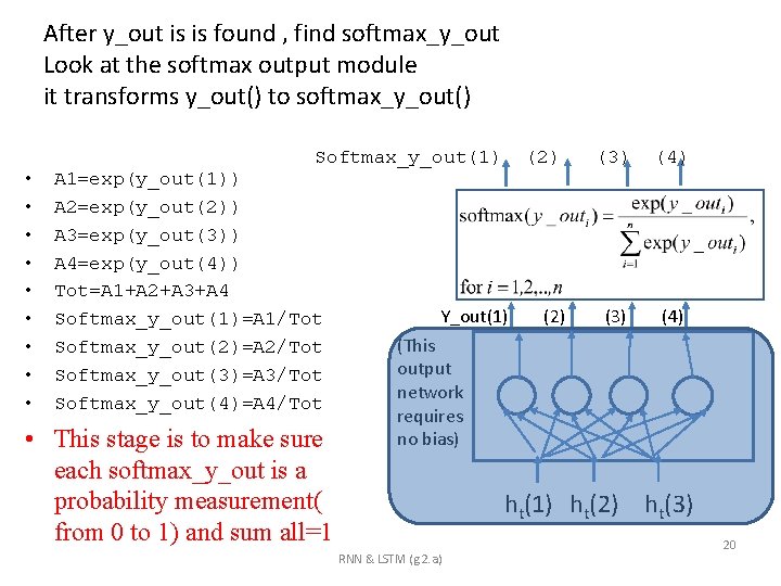
After y_out is is found , find softmax_y_out Look at the softmax output module it transforms y_out() to softmax_y_out() • • • Softmax_y_out(1) A 1=exp(y_out(1)) A 2=exp(y_out(2)) A 3=exp(y_out(3)) A 4=exp(y_out(4)) Tot=A 1+A 2+A 3+A 4 Softmax_y_out(1)=A 1/Tot Softmax_y_out(2)=A 2/Tot Softmax_y_out(3)=A 3/Tot Softmax_y_out(4)=A 4/Tot • This stage is to make sure each softmax_y_out is a probability measurement( from 0 to 1) and sum all=1 Y_out(1) (2) (3) (4) (This output network requires no bias) ht(1) ht(2) RNN & LSTM (g. 2. a) ht(3) 20

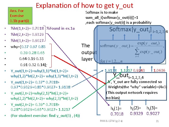
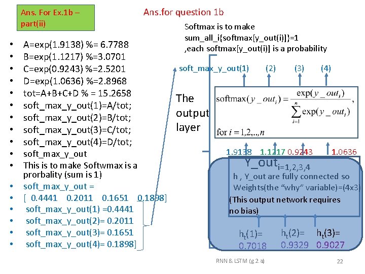
Ans. For Exercise 0. 1 b part(i) • • • Explanation of how to get y_out %ht(1, t=2)= 0. 7018 %Found in ex. 1 a %ht(2, t=2)= 0. 9329 %ht(3, t=2)= 0. 9027 why=[0. 37 0. 97 0. 83 0. 39 0. 28 0. 65 0. 64 0. 19 0. 33 0. 91 0. 32 0. 14]; Y_out(1, t=2)=why(1, 1)*ht(1, t=2)+ why(1, 2)*ht(2, t=2)+ why(1, 3)*ht(3, t=2) Y_out(1, t=2)= 0. 37* 0. 7018+ 0. 97*0. 9329+0. 83*0. 9027= 1. 9138 Y_out(2, t=2)=why(2, 1)*ht(2, t=2)+ why(2, 2)*ht(2, t=2)+ why(2, 3)*ht(3, t=2) Y_out(2, t=2)= 0. 39* 0. 7018+ 0. 28*0. 9329+0. 65*0. 9027= 1. 1217 (For student exercise: find y_out(3) , (4)) Softmax is to make sum_all_i{softmax[y_out(i)]}=1 , each softmax[y_out(i)] is a probability Softmax[y_outi] i=1, 2, 3, 4 The output layer 1. 9138 1. 1217 0. 9243 Y_outi=1, 2, 3, 4 1. 0636 h , Y_out are fully connected so Weights(the “why” variable)=(4 x 3) (This output network requires no bias) ht(1)= 0. 7018 RNN & LSTM (g. 2. a) ht(2)= ht(3)= 0. 9329 0. 9027 21

Ans. For Ex. 1 b – part(ii) • • • • • A=exp(1. 9138) %= 6. 7788 B=exp(1. 1217) %=3. 0701 C=exp(0. 9243) %=2. 5201 D=exp(1. 0636) %=2. 8968 tot=A+B+C+D % = 15. 2658 soft_max_y_out(1)=A/tot; soft_max_y_out(2)=B/tot; soft_max_y_out(3)=C/tot; soft_max_y_out(4)=D/tot; Ans. for question 1 b soft_max_y_out This is to make Softwmax is a prorbality (sum is 1) soft_max_y_out = [ 0. 4441 0. 2011 0. 1651 0. 1898] soft_max_y_out(1) =0. 4441 soft_max_y_out(2)= 0. 2011 soft_max_y_out(3)= 0. 1651 soft_max_y_out(4)= 0. 1898] Softmax is to make sum_all_i{softmax[y_out(i)]}=1 , each softmax[y_out(i)] is a probability soft_max_y_out(1) (2) (3) (4) The output layer 1. 9138 1. 1217 0. 9243 Y_outi=1, 2, 3, 4 1. 0636 h , Y_out are fully connected so Weights(the “why” variable)=(4 x 3) (This output network requires no bias) ht(1)= 0. 7018 RNN & LSTM (g. 2. a) ht(2)= ht(3)= 0. 9329 0. 9027 22

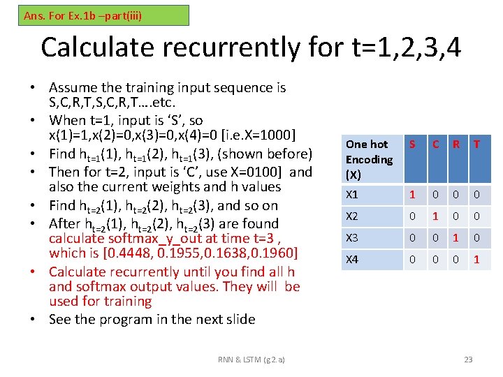
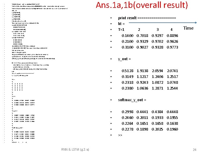
Ans. For Ex. 1 b –part(iii) Calculate recurrently for t=1, 2, 3, 4 • Assume the training input sequence is S, C, R, T, S, C, R, T…. etc. • When t=1, input is ‘S’, so x(1)=1, x(2)=0, x(3)=0, x(4)=0 [i. e. X=1000] • Find ht=1(1), ht=1(2), ht=1(3), (shown before) • Then for t=2, input is ‘C’, use X=0100] and also the current weights and h values • Find ht=2(1), ht=2(2), ht=2(3), and so on • After ht=2(1), ht=2(2), ht=2(3) are found calculate softmax_y_out at time t=3 , which is [0. 4448, 0. 1955, 0. 1638, 0. 1960] • Calculate recurrently until you find all h and softmax output values. They will be used for training • See the program in the next slide RNN & LSTM (g. 2. a) One hot Encoding (X) S C R T X 1 1 0 0 0 X 2 0 1 0 0 X 3 0 0 1 0 X 4 0 0 0 1 23

• • • • • • • • • • • • • • • • • %Matlab. Demo rnn 4 b. m modified f 2021 Feb 17 %https: //stackoverflow. com/questions/50050056/simple-rnn-example-showing-numerics %https: //www. analyticsvidhya. com/blog/2017/12/introduction-to-recurrent-neural-networks/ clear, clc in_S=[1 0 0 0]'; in_C=[0 1 0 0]'; in_R=[0 0 1 0]'; in_T=[0 0 0 1]'; X=[in_S, in_C, in_R, in_T]; %assume whx, whh, why are initialised at t=1 as whx=[0. 28 0. 84 0. 57 0. 48 0. 90 0. 87 0. 69 0. 18 0. 53 0. 09 0. 55 0. 49]; whh =[0. 11 0. 12 0. 13 0. 21 0. 24 0. 26 0. 31 0. 34 0. 36]; why=[0. 37 0. 97 0. 83 0. 39 0. 28 0. 65 0. 64 0. 19 0. 33 0. 91 0. 32 0. 14]; bias=[0. 51, 0. 62, 0. 73]'; %bias initialised ht(: , 1)=[0. 11 0. 21 0. 31]'; %assume ht has value initally at t=1 %Forward pass only %for t = 1: length(in)-1 % %(y_out not feedback to network, only h feeback to network) y_out(: , 1)=why*ht(: , 1); %the outputs at t=1 (inital value) softmax_y_out(: , 1)=softmax(y_out(: , 1)); %the outputs at t=1(inital value) for t = 1: 3 % assume we want to see 3 steps ht(: , t+1)=tanh( whx*X(: , t)+whh*ht(: , t)+bias); %recurrent layer y_out(: , t+1)=why*ht(: , t+1) ; softmax_y_out(: , t+1)=softmax(y_out(: , t+1)); %output layer end %'print result ==========‘ X, ht, y_out, softmax_y_out %X= % % 1 0 0 0 % 0 1 0 0 % 0 0 1 0 % 0 0 0 1 % % % ht = % % 0. 1100 0. 7002 % 0. 2100 0. 9321 % 0. 3100 0. 9009 % % % y_out = % % 0. 5017 1. 9110 % 0. 3032 1. 1196 % 0. 2126 0. 9225 % 0. 2107 1. 0615 % % % softmax_y_out = % % 0. 3015 0. 4438 % 0. 2472 0. 2012 % 0. 2258 0. 1652 % 0. 2254 0. 1898 % % %t= 1 2 3 2. 0741 1. 2517 1. 0747 1. 2544 0. 4383 0. 1933 0. 1658 0. 2025 0. 4448 0. 1955 0. 1638 0. 1960 • • • print result ========== ht = T=1 2 3 4 0. 1400 0. 7018 0. 9297 0. 8896 0. 2100 0. 9329 0. 9702 0. 9626 0. 3100 0. 9027 0. 9328 0. 9773 • y_out = • • 0. 9297 0. 8896 0. 9702 0. 9626 0. 9326 0. 9773 2. 0591 1. 2404 1. 0871 1. 2870 Ans. 1 a, 1 b(overall result) 0. 5128 0. 3149 0. 2318 0. 2380 1. 9138 1. 1217 0. 9243 1. 0636 • softmax_y_out = • • • 0. 2998 0. 2460 0. 2264 0. 2278 >> 0. 4441 0. 2011 0. 1651 0. 1898 2. 0594 1. 2406 1. 0872 1. 2871 2. 0741 1. 2517 1. 0748 1. 2544 0. 4384 0. 1933 0. 1658 0. 2025 0. 4448 0. 1955 0. 1638 0. 1960 Time 4 RNN & LSTM (g. 2. a) 24

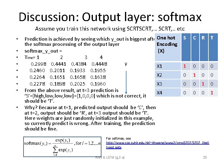
Discussion: Output layer: softmax Assume you train this network using SCRT, … SCRT, . . etc • • • Prediction is achieved by seeing which y_out is biggest after. One hot the softmax processing of the output layer Encoding softmax_y_out = (X) Time= 1 2 3 4 y 0. 2998 0. 4441 0. 4384 0. 4448 X 1 0. 2460 0. 2011 0. 1933 0. 1955 X 2 0. 2264 0. 1651 0. 1658 0. 1638 0. 2278 0. 1898 0. 2025 0. 1960 X 3 From the above result, at t=3 prediction is X 4 ‘S’=[high, low, low]=[1, 0, 0, 0] which is not correct, it should be ‘T’. Why? Because at t=1, predicted output should be ‘C’, then at t=2, output should be ‘R’, at t=3 output should be ‘T’. Here weights are just randomly initialized in this example, so currently predict is wrong. After training, the prediction should be fine. S C R T 1 0 0 0 0 1 For softmax, see http: //www. cse. cuhk. edu. hk/~khwong/www 2/cmsc 5707/5707_likeli hood. pptx RNN & LSTM (g. 2. a) 25

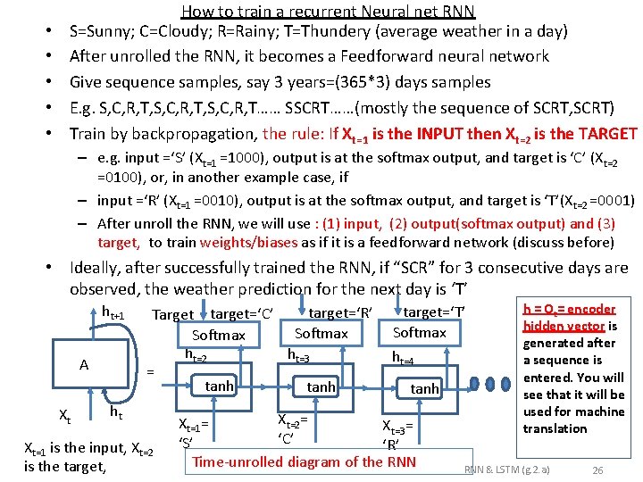
• • • How to train a recurrent Neural net RNN S=Sunny; C=Cloudy; R=Rainy; T=Thundery (average weather in a day) After unrolled the RNN, it becomes a Feedforward neural network Give sequence samples, say 3 years=(365*3) days samples E. g. S, C, R, T, S, C, R, T…… SSCRT……(mostly the sequence of SCRT, SCRT) Train by backpropagation, the rule: If Xt=1 is the INPUT then Xt=2 is the TARGET – e. g. input =‘S’ (Xt=1 =1000), output is at the softmax output, and target is ‘C’ (Xt=2 =0100), or, in another example case, if – input =‘R’ (Xt=1 =0010), output is at the softmax output, and target is ‘T’(Xt=2 =0001) – After unroll the RNN, we will use : (1) input, (2) output(softmax output) and (3) target, to train weights/biases as if it is a feedforward network (discuss before) • Ideally, after successfully trained the RNN, if “SCR” for 3 consecutive days are observed, the weather prediction for the next day is ‘T’ ht+1 A Xt target=‘R’ Target target=‘C’ Softmax ht=2 ht=3 = tanh ht Xt=1 is the input, Xt=2 is the target, target=‘T’ Softmax ht=4 tanh Xt=2= Xt=1= Xt=3= ‘C’ ‘S’ ‘R’ Time-unrolled diagram of the RNN h = Ot= encoder hidden vector is generated after a sequence is entered. You will see that it will be used for machine translation RNN & LSTM (g. 2. a) 26

Problem with RNN: The vanishing gradient problem Ref: https: //hackernoon. com/exploding-and-vanishing-gradient-problem-math-behind-the-truth 6 bd 008 df 6 e 25 RNN & LSTM (g. 2. a) 27

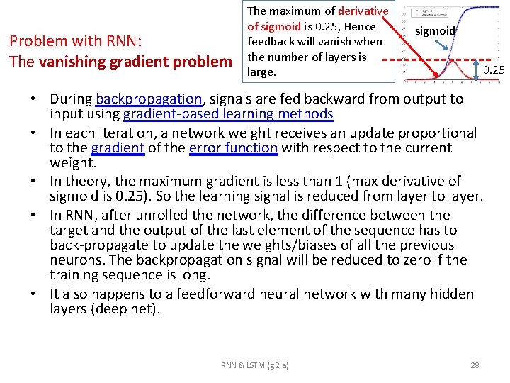
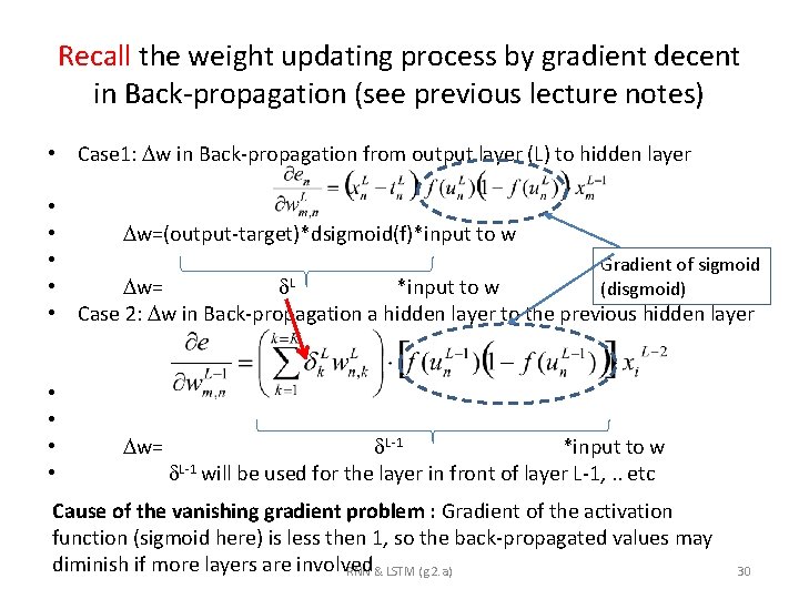
Problem with RNN: The vanishing gradient problem The maximum of derivative of sigmoid is 0. 25, Hence feedback will vanish when the number of layers is large. sigmoid 0. 25 • During backpropagation, signals are fed backward from output to input using gradient-based learning methods • In each iteration, a network weight receives an update proportional to the gradient of the error function with respect to the current weight. • In theory, the maximum gradient is less than 1 (max derivative of sigmoid is 0. 25). So the learning signal is reduced from layer to layer. • In RNN, after unrolled the network, the difference between the target and the output of the last element of the sequence has to back-propagate to update the weights/biases of all the previous neurons. The backpropagation signal will be reduced to zero if the training sequence is long. • It also happens to a feedforward neural network with many hidden layers (deep net). RNN & LSTM (g. 2. a) 28

https: //imiloainf. wordpress. com/2013/11/06/rectifier-nonlinearities/ https: //www. simonwenkel. com/2018/05/15/activation-functions-for-neural-networks. html#softplus Activation function choices Max. gradient of Signmoid is 0. 25, it will cause the vanishing gradient problem Relu is now very popular and shown to be working better other methods RNN & LSTM (g. 2. a) 29

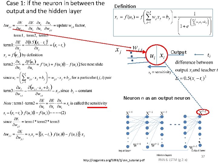
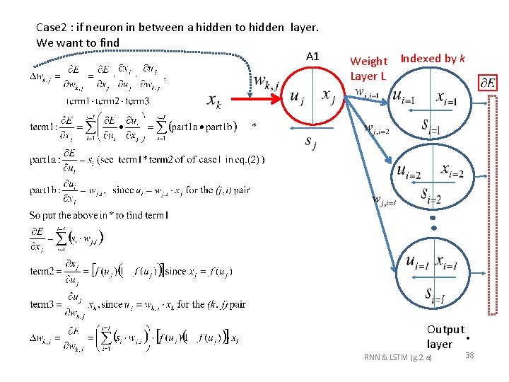
Recall the weight updating process by gradient decent in Back-propagation (see previous lecture notes) • Case 1: w in Back-propagation from output layer (L) to hidden layer • • w=(output-target)*dsigmoid(f)*input to w • Gradient of sigmoid L • w= *input to w (disgmoid) • Case 2: w in Back-propagation a hidden layer to the previous hidden layer • • w= L-1 *input to w L-1 will be used for the layer in front of layer L-1, . . etc Cause of the vanishing gradient problem : Gradient of the activation function (sigmoid here) is less then 1, so the back-propagated values may diminish if more layers are involved RNN & LSTM (g. 2. a) 30

To solve the vanishing gradient problem, LSTM adds C (cell state) • RNN has xi (input) and ht (output) only • In LSTM (Long Short Term Memory), add – Cell state (Ct) to solve gradient vanishing problem – In each time (t), updates • Ct=cell state (ranges from -1 to 1) • ht= output (ranges from 0 to 1) • The system learns Ct and ht together RNN & LSTM (g. 2. a) 31

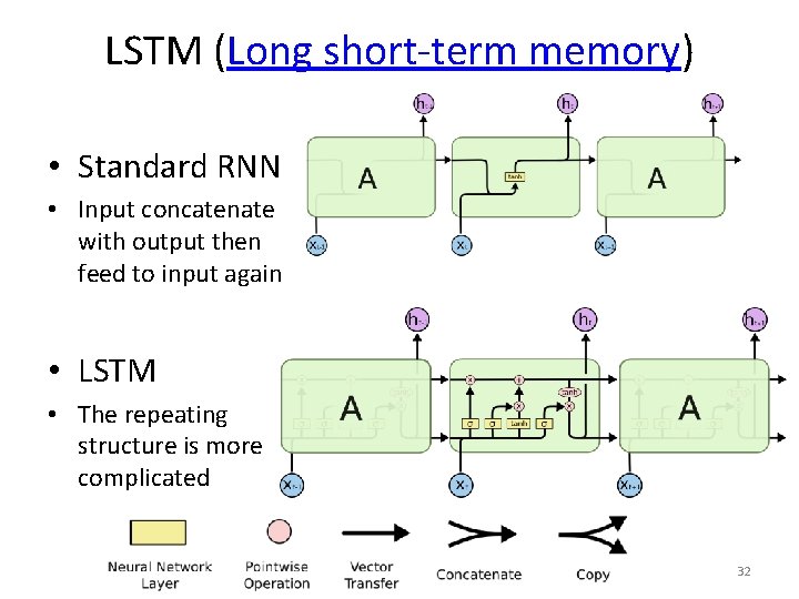
LSTM (Long short-term memory) • Standard RNN • Input concatenate with output then feed to input again • LSTM • The repeating structure is more complicated RNN & LSTM (g. 2. a) 32

Summary • Introduced the idea of Recurrent Neural Networks RNN • Gave and explained an example of RNN & LSTM (g. 2. a) 33

References • • • Deep Learning Book. http: //www. deeplearningbook. org/ • • Papers: Fully convolutional networks for semantic segmentation by J Long, Sequence to sequence learning with neural networks by tutorials http: //colah. github. io/posts/2015 -08 -Understanding-LSTMs/ https: //github. com/terryum/awesome-deep-learning-papers • • • turtorial: https: //theneuralperspective. com/tag/tutorials/ • • • RNN encoder-decoder https: //theneuralperspective. com/2016/11/20/recurrent-neural-networks-rnn-part-3 -encoder-decoder/ sequence to sequence model E Shelhamer, T Darrell I Sutskever, O Vinyals, QV Le - – – – https: //arxiv. org/pdf/1703. 01619. pdf https: //indico. io/blog/sequence-modeling-neuralnets-part 1/ https: //medium. com/towards-data-science/lstm-by-example-using-tensorflow-feb 0 c 1968537 https: //google. github. io/seq 2 seq/nmt/ https: //chunml. github. io/Chun. ML. github. io/project/Sequence-To-Sequence/ parameters of lstm • • https: //stackoverflow. com/questions/38080035/how-to-calculate-the-number-of-parameters-of-an-lstm-network https: //datascience. stackexchange. com/questions/10615/number-of-parameters-in-an-lstm-model https: //stackoverflow. com/questions/38080035/how-to-calculate-the-number-of-parameters-of-an-lstm-network https: //www. quora. com/What-is-the-meaning-of-%E 2%80%9 CThe-number-of-units-in-the-LSTM-cell https: //www. quora. com/In-LSTM-how-do-you-figure-out-what-size-the-weights-are-supposed-to-be http: //kbullaughey. github. io/lstm-play/lstm/ (batch size example) – feedback – Numerical examples • • https: //medium. com/@aidangomez/let-s-do-this-f 9 b 699 de 31 d 9 https: //blog. aidangomez. ca/2016/04/17/Backpropogating-an-LSTM-A-Numerical-Example/ https: //karanalytics. wordpress. com/2017/06/06/sequence-modelling-using-deep-learning/ http: //monik. in/a-noobs-guide-to-implementing-rnn-lstm-using-tensorflow/ RNN & LSTM (g. 2. a) 34

Appendix RNN & LSTM (g. 2. a) 35

Appendix 1 a: Using Square error for output measurement RNN & LSTM (g. 2. a) 36

Case 1: if the neuron in between the output and the hidden layer Definition Output ti Neuron n as an output neuron • http: //cogprints. org/5869/1/cnn_tutorial. pdf RNN & LSTM (g. 2. a) 37

Case 2 : if neuron in between a hidden to hidden layer. We want to find A 1 Weight Layer L Indexed by k Output layer • RNN & LSTM (g. 2. a) 38

Appendix 1 b Using softmax with cross-entropy_loss for a 2 -classifier (single output neuron) RNN & LSTM (g. 2. a) 39

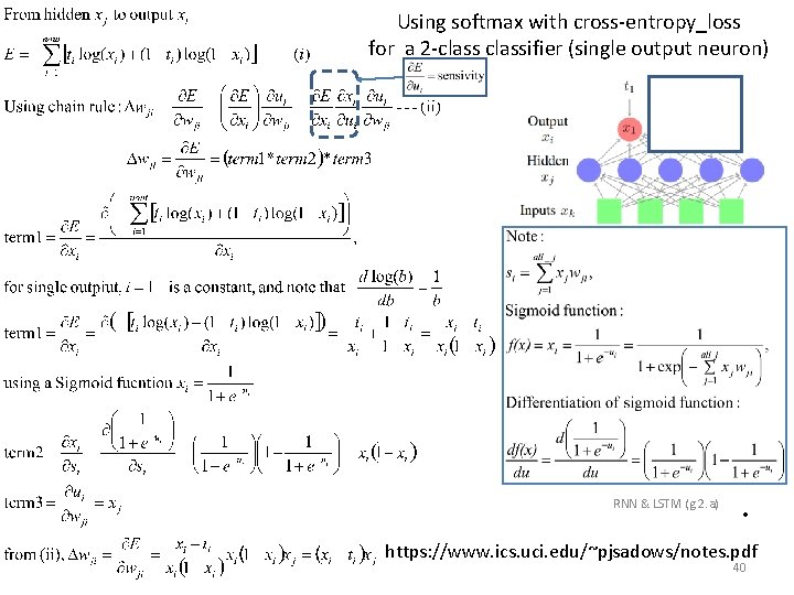
Using softmax with cross-entropy_loss for a 2 -classifier (single output neuron) RNN & LSTM (g. 2. a) • https: //www. ics. uci. edu/~pjsadows/notes. pdf 40

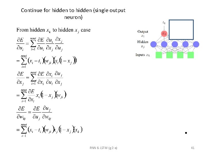
Continue for hidden to hidden (single output neuron) • RNN & LSTM (g. 2. a) 41