Alignment Matrix vs Distance Matrix Sequence a gene

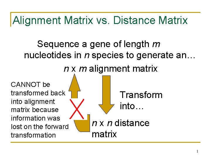
Alignment Matrix vs. Distance Matrix Sequence a gene of length m nucleotides in n species to generate an… n x m alignment matrix CANNOT be transformed back into alignment matrix because information was lost on the forward transformation Transform into… n x n distance matrix 1

Character-Based Tree Reconstruction • Better technique: • Character-based reconstruction algorithms use the n x m alignment matrix (n = # species, m = #characters) directly instead of using distance matrix. • GOAL: determine what character strings at internal nodes would best explain the character strings for the n observed species 2

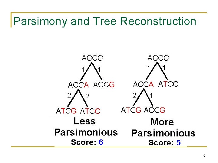
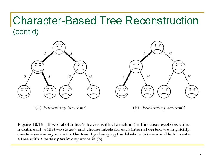
Character-Based Tree Reconstruction (cont’d) • Characters may be nucleotides, where A, G, C, T are states of this character. Other characters may be the # of eyes or legs or the shape of a beak or a fin. • By setting the length of an edge in the tree to the Hamming distance, we may define the parsimony score of the tree as the sum of the lengths (weights) of the edges 3

Parsimony Approach to Evolutionary Tree Reconstruction • • • Applies Occam’s razor principle to identify the simplest explanation for the data Assumes observed character differences resulted from the fewest possible mutations Seeks the tree that yields lowest possible parsimony score - sum of cost of all mutations found in the tree 4

Parsimony and Tree Reconstruction 5

Character-Based Tree Reconstruction (cont’d) 6

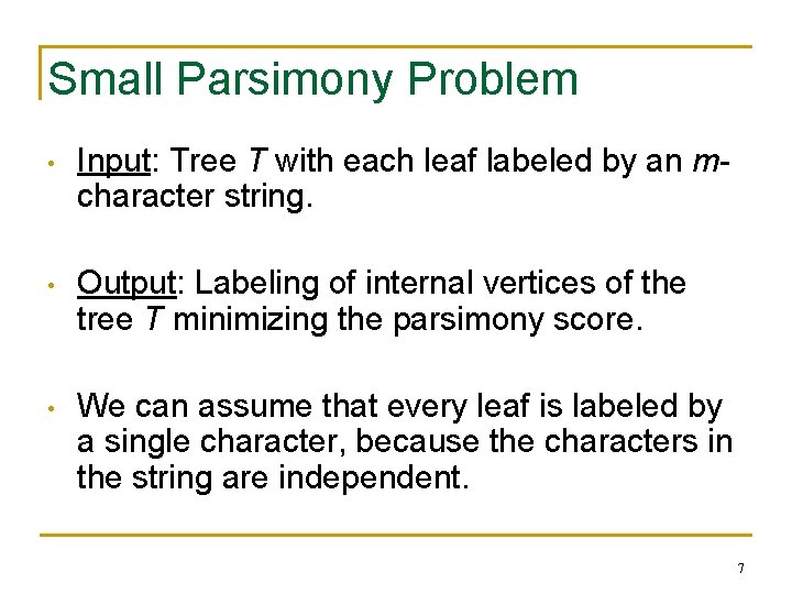
Small Parsimony Problem • Input: Tree T with each leaf labeled by an mcharacter string. • Output: Labeling of internal vertices of the tree T minimizing the parsimony score. • We can assume that every leaf is labeled by a single character, because the characters in the string are independent. 7

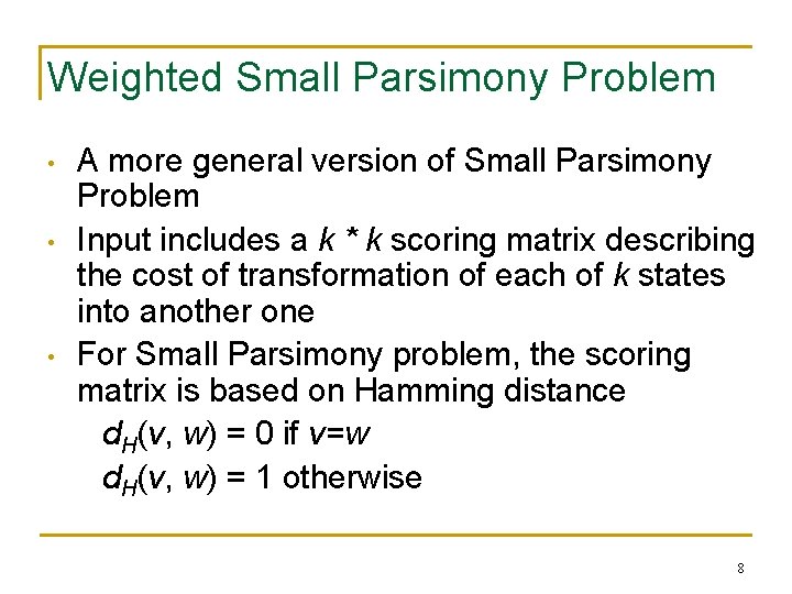
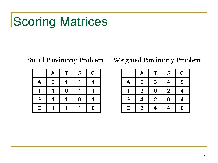
Weighted Small Parsimony Problem • • • A more general version of Small Parsimony Problem Input includes a k * k scoring matrix describing the cost of transformation of each of k states into another one For Small Parsimony problem, the scoring matrix is based on Hamming distance d. H(v, w) = 0 if v=w d. H(v, w) = 1 otherwise 8

Scoring Matrices Small Parsimony Problem A T G C A 0 1 1 1 T 1 0 1 G 1 1 C 1 1 Weighted Parsimony Problem A T G C A 0 3 4 9 1 T 3 0 2 4 0 1 G 4 2 0 4 1 0 C 9 4 4 0 9

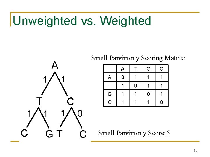
Unweighted vs. Weighted Small Parsimony Scoring Matrix: A T G C A 0 1 1 1 T 1 0 1 1 G 1 1 0 1 C 1 1 1 0 Small Parsimony Score: 5 10

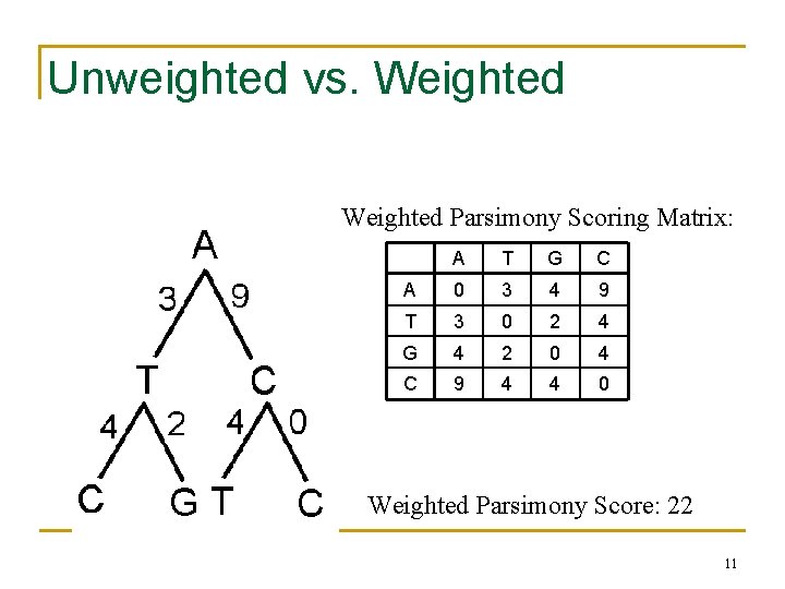
Unweighted vs. Weighted Parsimony Scoring Matrix: A T G C A 0 3 4 9 T 3 0 2 4 G 4 2 0 4 C 9 4 4 0 Weighted Parsimony Score: 22 11

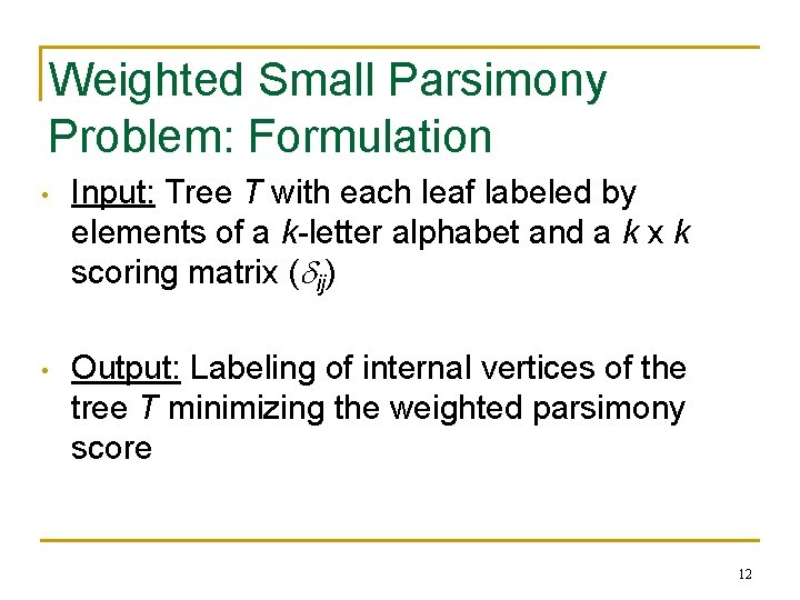
Weighted Small Parsimony Problem: Formulation • Input: Tree T with each leaf labeled by elements of a k-letter alphabet and a k x k scoring matrix ( ij) • Output: Labeling of internal vertices of the tree T minimizing the weighted parsimony score 12

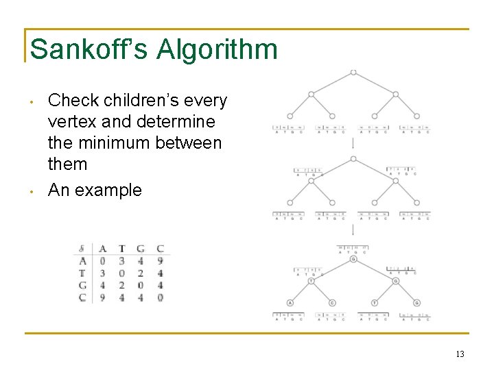
Sankoff’s Algorithm • • Check children’s every vertex and determine the minimum between them An example 13

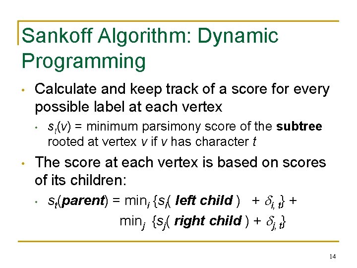
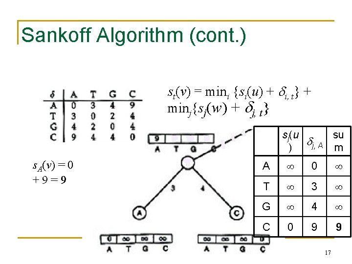
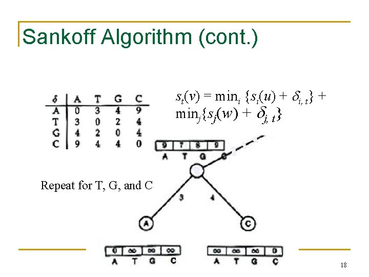
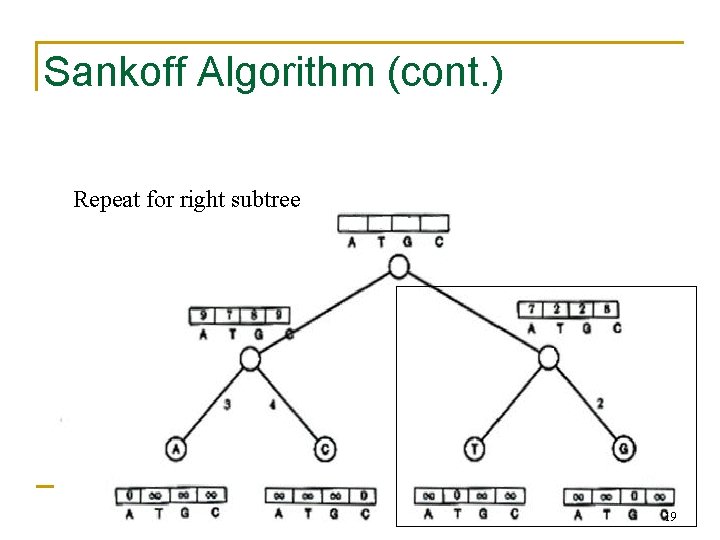
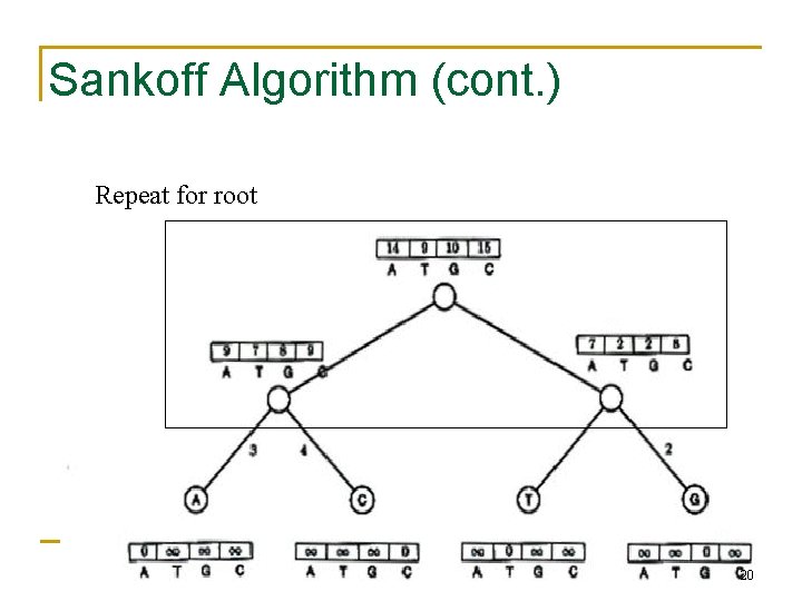
Sankoff Algorithm: Dynamic Programming • Calculate and keep track of a score for every possible label at each vertex • • st(v) = minimum parsimony score of the subtree rooted at vertex v if v has character t The score at each vertex is based on scores of its children: • st(parent) = mini {si( left child ) + i, t} + minj {sj( right child ) + j, t} 14

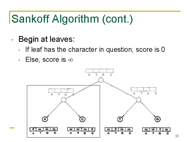
Sankoff Algorithm (cont. ) • Begin at leaves: • • If leaf has the character in question, score is 0 Else, score is 15

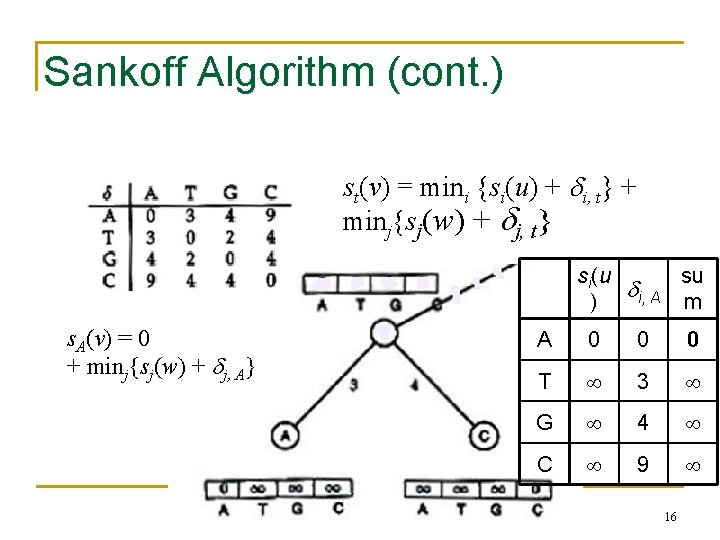
Sankoff Algorithm (cont. ) st(v) = mini {si(u) + i, t} + minj{sj(w) + j, t} si(u su i, A m ) s. A(v) = 0 mini{si(u) + i, A} + minj{sj(w) + j, A} A 0 0 0 T 3 G 4 C 9 16

Sankoff Algorithm (cont. ) st(v) = mini {si(u) + i, t} + minj{sj(w) + j, t} sj(u su j, A m ) s. A(v) = 0 mini{si(u) + i, A} + 9 min = 9 j{sj(w) + j, A} A 0 T 3 G 4 C 0 9 9 17

Sankoff Algorithm (cont. ) st(v) = mini {si(u) + i, t} + minj{sj(w) + j, t} Repeat for T, G, and C 18

Sankoff Algorithm (cont. ) Repeat for right subtree 19

Sankoff Algorithm (cont. ) Repeat for root 20

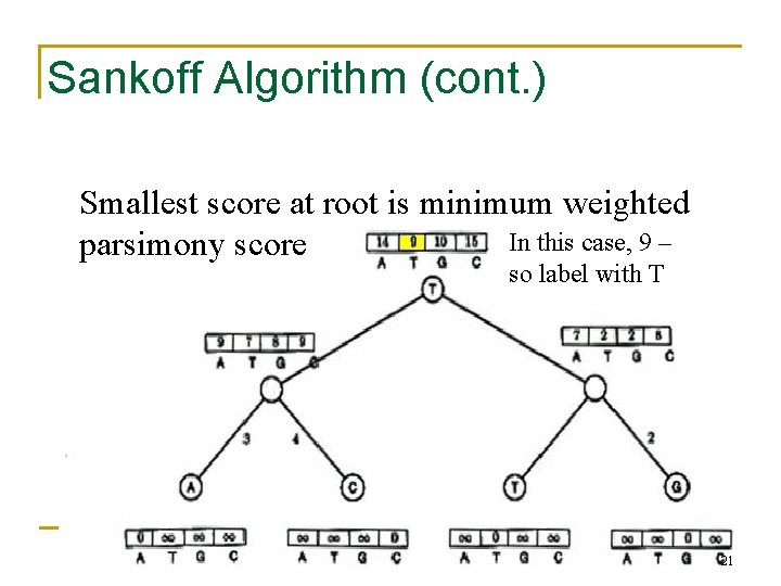
Sankoff Algorithm (cont. ) Smallest score at root is minimum weighted In this case, 9 – parsimony score so label with T 21

Sankoff Algorithm: Traveling down the Tree • • The scores at the root vertex have been computed by going up the tree After the scores at root vertex are computed the Sankoff algorithm moves down the tree and assign each vertex with optimal character. 22

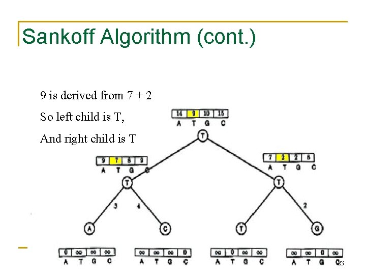
Sankoff Algorithm (cont. ) 9 is derived from 7 + 2 So left child is T, And right child is T 23

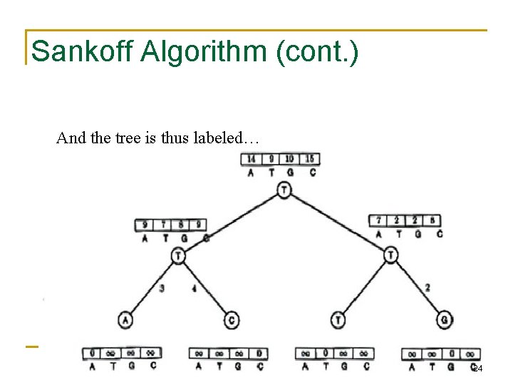
Sankoff Algorithm (cont. ) And the tree is thus labeled… 24

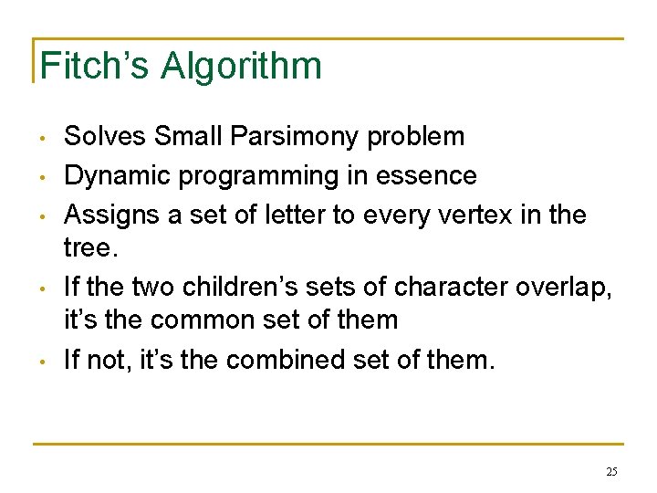
Fitch’s Algorithm • • • Solves Small Parsimony problem Dynamic programming in essence Assigns a set of letter to every vertex in the tree. If the two children’s sets of character overlap, it’s the common set of them If not, it’s the combined set of them. 25

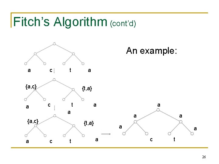
Fitch’s Algorithm (cont’d) An example: a c t a {a, c} a {t, a} c t a a {a, c} a a a {t, a} c t a a c t 26

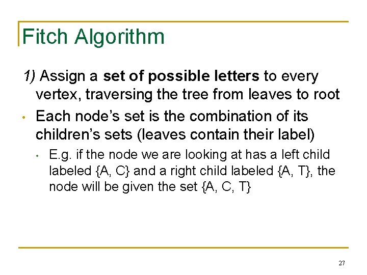
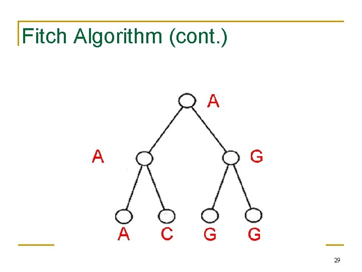
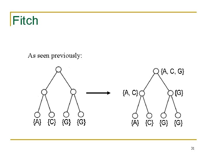
Fitch Algorithm 1) Assign a set of possible letters to every vertex, traversing the tree from leaves to root • Each node’s set is the combination of its children’s sets (leaves contain their label) • E. g. if the node we are looking at has a left child labeled {A, C} and a right child labeled {A, T}, the node will be given the set {A, C, T} 27

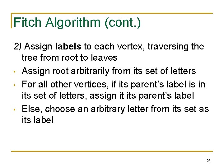
Fitch Algorithm (cont. ) 2) Assign labels to each vertex, traversing the tree from root to leaves • Assign root arbitrarily from its set of letters • For all other vertices, if its parent’s label is in its set of letters, assign it its parent’s label • Else, choose an arbitrary letter from its set as its label 28

Fitch Algorithm (cont. ) 29

Fitch vs. Sankoff • Both have an O(nk) runtime • Are they actually different? • Let’s compare … 30

Fitch As seen previously: 31

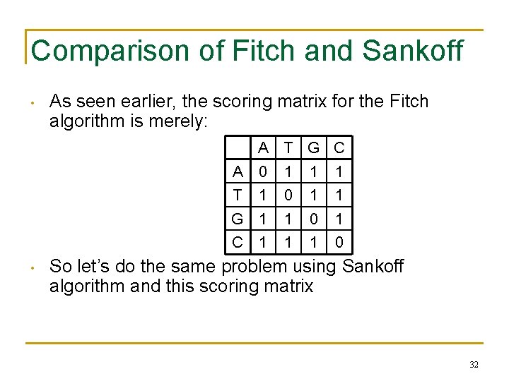
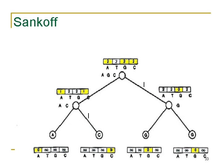
Comparison of Fitch and Sankoff • As seen earlier, the scoring matrix for the Fitch algorithm is merely: A T G C • A 0 1 1 1 T 1 0 1 1 G 1 1 0 1 C 1 1 1 0 So let’s do the same problem using Sankoff algorithm and this scoring matrix 32

Sankoff 33

Sankoff vs. Fitch • • The Sankoff algorithm gives the same set of optimal labels as the Fitch algorithm For Sankoff algorithm, character t is optimal for vertex v if st(v) = min 1<i<ksi(v) • Denote the set of optimal letters at vertex v as S(v) • If S(left child) and S(right child) overlap, S(parent) is the intersection • Else it’s the union of S(left child) and S(right child) • • This is also the Fitch recurrence The two algorithms are identical 34

Large Parsimony Problem • • Input: An n x m matrix M describing n species, each represented by an m-character string Output: A tree T with n leaves labeled by the n rows of matrix M, and a labeling of the internal vertices such that the parsimony score is minimized over all possible trees and all possible labelings of internal vertices 35

Large Parsimony Problem (cont. ) • Possible search space is huge, especially as n increases • • • Problem is NP-complete • • (2 n – 3)!! possible rooted trees (2 n – 5)!! possible unrooted trees Exhaustive search only possible w/ small n(< 10) Hence, branch and bound or heuristics used 36

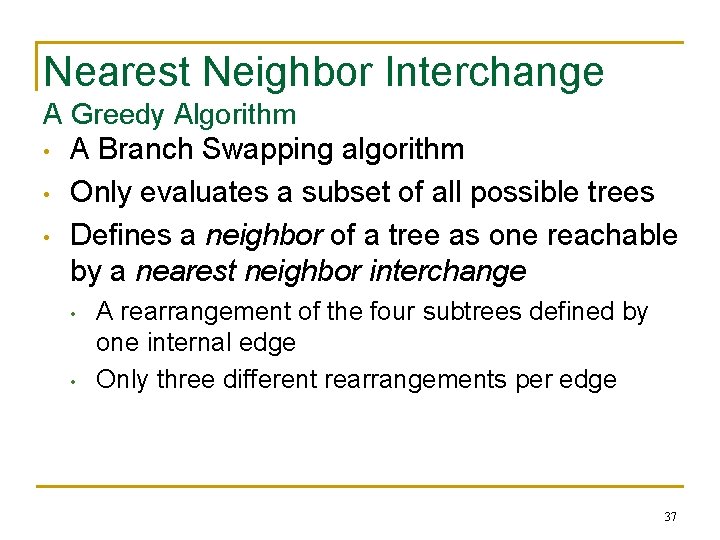
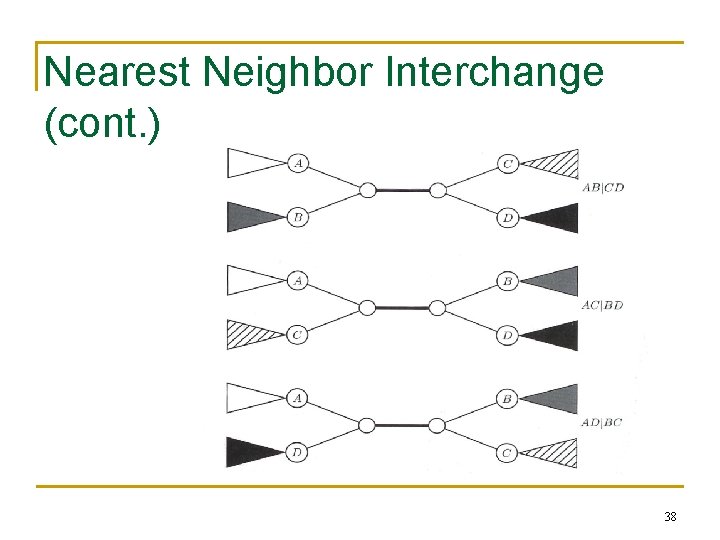
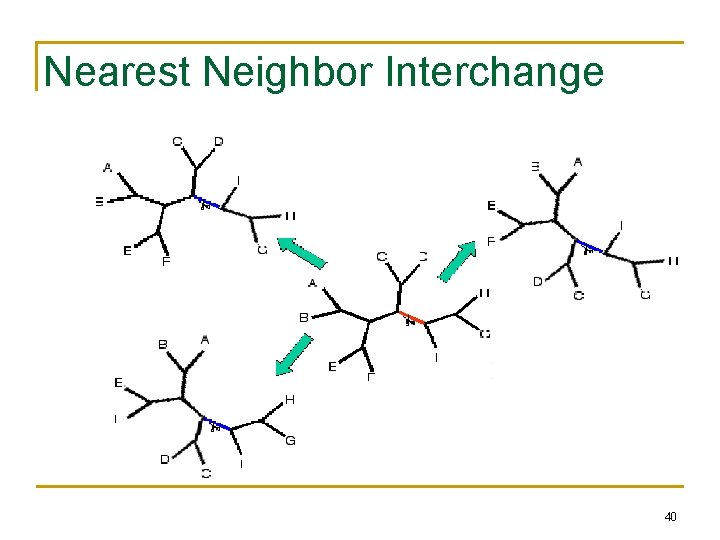
Nearest Neighbor Interchange A Greedy Algorithm • A Branch Swapping algorithm • Only evaluates a subset of all possible trees • Defines a neighbor of a tree as one reachable by a nearest neighbor interchange • • A rearrangement of the four subtrees defined by one internal edge Only three different rearrangements per edge 37

Nearest Neighbor Interchange (cont. ) 38

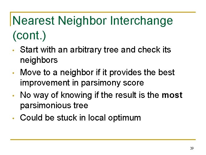
Nearest Neighbor Interchange (cont. ) • • Start with an arbitrary tree and check its neighbors Move to a neighbor if it provides the best improvement in parsimony score No way of knowing if the result is the most parsimonious tree Could be stuck in local optimum 39

Nearest Neighbor Interchange 40

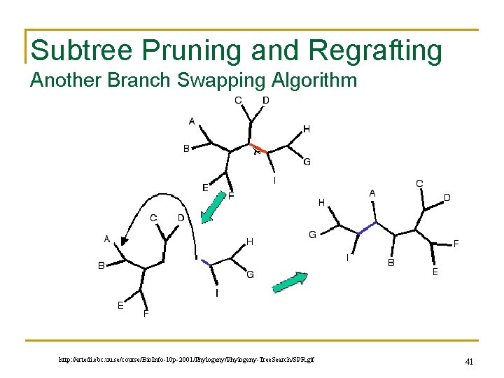
Subtree Pruning and Regrafting Another Branch Swapping Algorithm http: //artedi. ebc. uu. se/course/Bio. Info-10 p-2001/Phylogeny-Tree. Search/SPR. gif 41

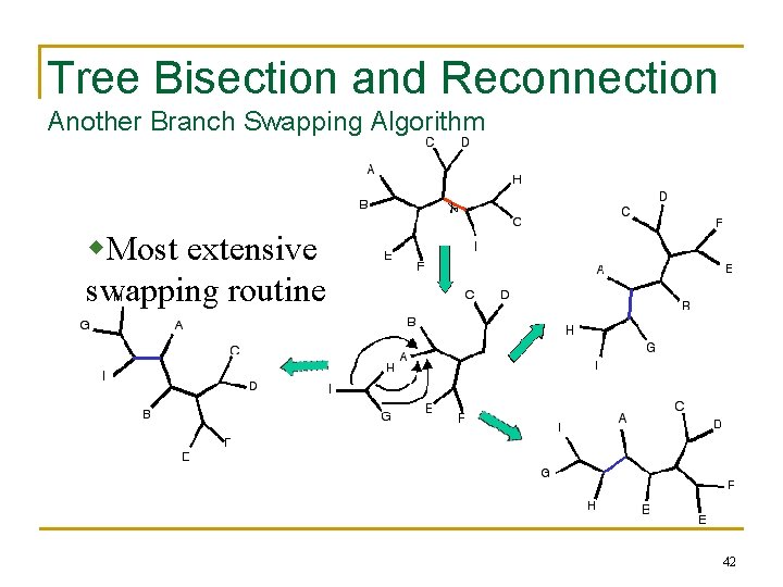
Tree Bisection and Reconnection Another Branch Swapping Algorithm w. Most extensive swapping routine 42

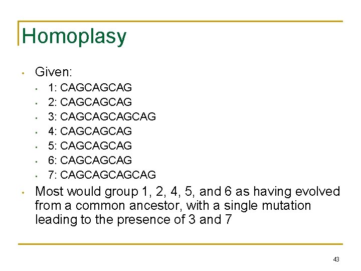
Homoplasy • Given: • • 1: CAGCAGCAG 2: CAGCAGCAG 3: CAGCAG 4: CAGCAGCAG 5: CAGCAGCAG 6: CAGCAGCAG 7: CAGCAG Most would group 1, 2, 4, 5, and 6 as having evolved from a common ancestor, with a single mutation leading to the presence of 3 and 7 43

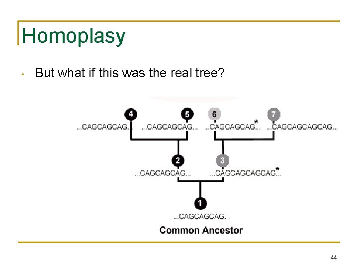
Homoplasy • But what if this was the real tree? 44

Homoplasy • • • 6 evolved separately from 4 and 5, but parsimony would group 4, 5, and 6 together as having evolved from a common ancestor Homoplasy: Independent (or parallel) evolution of same/similar characters Parsimony results minimize homoplasy, so if homoplasy is common, parsimony may give wrong results 45

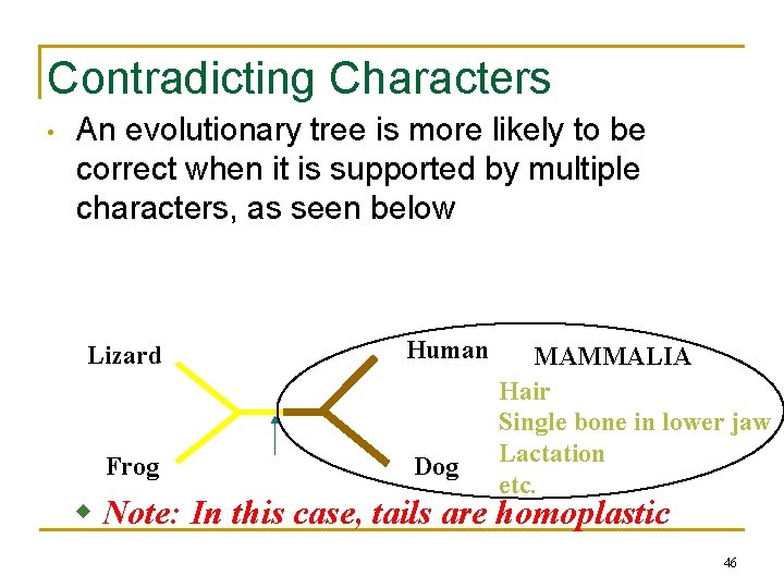
Contradicting Characters • An evolutionary tree is more likely to be correct when it is supported by multiple characters, as seen below Lizard Frog Human Dog MAMMALIA Hair Single bone in lower jaw Lactation etc. w Note: In this case, tails are homoplastic 46

Problems with Parsimony • • Important to keep in mind that reliance on purely one method for phylogenetic analysis provides incomplete picture When different methods (parsimony, distance -based, etc. ) all give same result, more likely that the result is correct 47

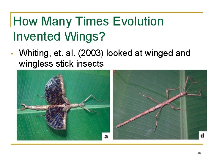
How Many Times Evolution Invented Wings? • Whiting, et. al. (2003) looked at winged and wingless stick insects 48

Reinventing Wings • • • Previous studies had shown winged wingless transitions Wingless winged transition much more complicated (need to develop many new biochemical pathways) Used multiple tree reconstruction techniques, all of which required reevolution of wings 49

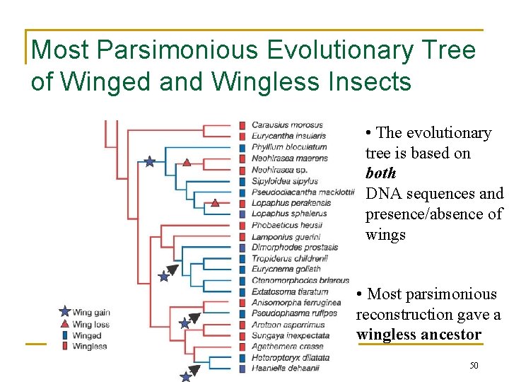
Most Parsimonious Evolutionary Tree of Winged and Wingless Insects • The evolutionary tree is based on both DNA sequences and presence/absence of wings • Most parsimonious reconstruction gave a wingless ancestor 50

Will Wingless Insects Fly Again? • Since the most parsimonious reconstructions all required the re-invention of wings, it is most likely that wing developmental pathways are conserved in wingless stick insects 51