Pairwise Sequence Alignment Pairwise alignments in the 1950

Pairwise Sequence Alignment

Pairwise alignments in the 1950 s b-corticotropin (sheep) Corticotropin A (pig) Oxytocin Vasopressin ala gly glu asp gly ala glu asp glu CYIQNCPLG CYFQNCPRG

globins: a- b- myoglobin Early example of sequence alignment: globins (1961) H. C. Watson and J. C. Kendrew, “Comparison Between the Amino-Acid Sequences of Sperm Whale Myoglobin and of Human Hæmoglobin. ” Nature 190: 670 -672, 1961.

Pairwise sequence alignment is the most fundamental operation of bioinformatics • It is used to decide if two proteins (or genes) are related structurally or functionally • It is used to identify domains or motifs that are shared between proteins • It is the basis of BLAST searching (next topic) • It is used in the analysis of genomes

Pairwise alignment: protein sequences can be more informative than DNA • protein is more informative (20 vs 4 characters); many amino acids share related biophysical properties • codons are degenerate: changes in the third position often do not alter the amino acid that is specified • protein sequences offer a longer “look-back” time (protein sequence comparisons can identify homologous sequences from organisms that last shared a common ancestor 1 billion years ago vs. 600 million years for DNA) • DNA sequences can be translated into protein, and then used in pairwise alignments

Standard Genetic Code

Pairwise alignment: protein sequences can be more informative than DNA • Many times, DNA alignments are appropriate --to confirm the identity of a c. DNA --to study noncoding regions of DNA --to study DNA polymorphisms --example: Neanderthal vs modern human DNA Query: 181 catcaactacaactccaaagacacccttacacccactaggatatcaacaaacctacccac 240 |||||| |||||||||||||||| Sbjct: 189 catcaactgcaaccccaaagccacccct-cacccactaggatatcaacaaacctacccac 247

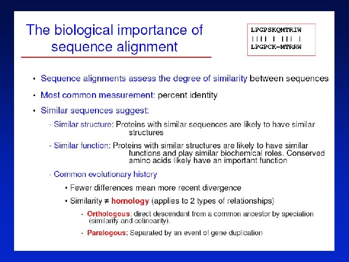
Definition: pairwise alignment Pairwise alignment The process of lining up two sequences to achieve maximal levels of identity (and conservation, in the case of amino acid sequences) for the purpose of assessing the degree of similarity and the possibility of homology.

Definition: homology Homology Similarity attributed to descent from a common ancestor. Two types of homology Orthologs Homologous sequences in different species that arose from a common ancestral gene during speciation; may or may not be responsible for a similar function. Paralogs Homologous sequences within a single species that arose by gene duplication.

These are homologous proteins: very similar structure, however limited amino acid identity. Beta globin (NP_000509) 2 HHB myoglobin (NP_005359) 2 MM 1

Orthologs: members of a gene (protein) family in various organisms. This tree shows globin orthologs.

Paralogs: members of a gene (protein) family within a species. This tree shows human globin paralogs.

Orthologs and paralogs are often viewed in a single tree Source: NCBI

General approach to pairwise alignment • Choose two sequences • Select an algorithm that generates a score • Allow gaps (insertions, deletions) • Score reflects degree of similarity • Alignments can be global or local • Estimate probability that the alignment occurred by chance

Calculation of an alignment score

Find BLAST from the home page of NCBI and select protein BLAST…

Choose align two or more sequences…

Enter the two sequences (as accession numbers or in the fasta format) and click BLAST. Optionally select “Algorithm parameters” and note the matrix option.

Pairwise alignment result of human beta globin and myoglobin Myoglobin Ref. Seq Query = HBB Subject = MB Information about this alignment: score, expect value, identities, positives, gaps… Middle row displays identities; + sign for similar matches

Pairwise alignment result of human beta globin and myoglobin: the score is a sum of match, mismatch, gap creation, and gap extension scores

Pairwise alignment result of human beta globin and myoglobin: the score is a sum of match, mismatch, gap creation, and gap extension scores V matching V earns +4 T matching L earns -1 These scores come from a “scoring matrix”!

Definitions: identity, similarity, conservation Identity The extent to which two (nucleotide or amino acid) sequences are invariant. Similarity The extent to which nucleotide or protein sequences are related. It is based upon identity plus conservation. Conservation Changes at a specific position of an amino acid or (less commonly, DNA) sequence that preserve the physico-chemical properties of the original residue.

Mind the gaps First gap position scores -11 Second gap position scores -1 Gap creation tends to have a large negative score; Gap extension involves a small penalty

Gaps • Positions at which a letter is paired with a null are called gaps. • Gap scores are typically negative. • Since a single mutational event may cause the insertion or deletion of more than one residue, the presence of a gap is ascribed more significance than the length of the gap. Thus there are separate penalties for: gap creation and gap extension. • In BLAST, it is rarely necessary to change gap values from the default.

Pairwise alignment of retinol-binding protein and b-lactoglobulin: Example of an alignment with internal, terminal gaps 1 MKWVWALLLLAAWAAAERDCRVSSFRVKENFDKARFSGTWYAMAKKDPEG 50 RBP. ||| |. |. . . | : . ||||. : | : 1. . . MKCLLLALALTCGAQALIVT. . QTMKGLDIQKVAGTWYSLAMAASD. 44 lactoglobulin 51 LFLQDNIVAEFSVDETGQMSATAKGRVR. LLNNWD. . VCADMVGTFTDTE 97 RBP : | | : : |. |. || |: || |. 45 ISLLDAQSAPLRV. YVEELKPTPEGDLEILLQKWENGECAQKKIIAEKTK 93 lactoglobulin 98 DPAKFKMKYWGVASFLQKGNDDHWIVDTDYDTYAV. . . QYSC 136 RBP || ||. | : . |||| |. . | 94 IPAVFKIDALNENKVL. . . . VLDTDYKKYLLFCMENSAEPEQSLAC 135 lactoglobulin 137 RLLNLDGTCADSYSFVFSRDPNGLPPEAQKIVRQRQ. EELCLARQYRLIV 185 RBP. | | | : ||. | || | 136 QCLVRTPEVDDEALEKFDKALKALPMHIRLSFNPTQLEEQCHI. . . . 178 lactoglobulin

Pairwise alignment of retinol-binding protein from human (top) and rainbow trout (O. mykiss): Example of an alignment with few gaps 1. MKWVWALLLLA. AWAAAERDCRVSSFRVKENFDKARFSGTWYAMAKKDP 48 : : || || ||. ||. . | : |||: . | ||||| 1 MLRICVALCALATCWA. . . QDCQVSNIQVMQNFDRSRYTGRWYAVAKKDP 47. . . 49 EGLFLQDNIVAEFSVDETGQMSATAKGRVRLLNNWDVCADMVGTFTDTED 98 |||| ||: |||||. ||| : ||||: . ||. | || | 48 VGLFLLDNVVAQFSVDESGKMTATAHGRVIILNNWEMCANMFGTFEDTPD 97. . . 99 PAKFKMKYWGVASFLQKGNDDHWIVDTDYDTYAVQYSCRLLNLDGTCADS 148 ||||||: ||| ||: || ||||||: : ||||| ||: ||||. . ||||| | 98 PAKFKMRYWGAASYLQTGNDDHWVIDTDYDNYAIHYSCREVDLDGTCLDG 147. . . 149 YSFVFSRDPNGLPPEAQKIVRQRQEELCLARQYRLIVHNGYCDGRSERNLL 199 |||: ||| || |||| : . . |: |. || : | |: |: 148 YSFIFSRHPTGLRPEDQKIVTDKKKEICFLGKYRRVGHTGFCESS. . . 192

Pairwise sequence alignment allows us to look back billions of years ago (BYA) Origin of life 4 Earliest fossils Origin of Eukaryote/ eukaryotes archaea 3 2 Fungi/animal Plant/animal insects 1 When you do a pairwise alignment of homologous human and plant proteins, you are studying sequences that last shared a common ancestor 1. 5 billion years ago! 0

Multiple sequence alignment of glyceraldehyde 3 -phosphate dehydrogenases: example of extremely high conservation fly human plant bacterium yeast archaeon GAKKVIISAP GAKRVIISAP GAKKVVMTGP GAKKVVITAP GADKVLISAP SAD. APM. . F SKDNTPM. . F SS. TAPM. . F PKGDEPVKQL VCGVNLDAYK VMGVNHEKYD VVGVNEHTYQ VKGANFDKY. VMGVNEEKYT VYGVNHDEYD PDMKVVSNAS NSLKIISNAS PNMDIVSNAS AGQDIVSNAS SDLKIVSNAS GE. DVVSNAS CTTNCLAPLA CTTNCLAPLA CTTNSITPVA fly human plant bacterium yeast archaeon KVINDNFEIV KVIHDNFGIV KVVHEEFGIL KVINDNFGII KVINDAFGIE KVLDEEFGIN EGLMTTVHAT EGLMTTVHAI EGLMTTVHAT EGLMTTVHSL AGQLTTVHAY TATQKTVDGP TATQKTVDGP TGSQNLMDGP SGKLWRDGRG SMKDWRGGRG SHKDWRGGRT NGKP. RRRRA AAQNIIPAST ALQNIIPAST ASQNIIPSST ASGNIIPSST AAENIIPTST fly human plant bacterium yeast archaeon GAAKAVGKVI GAAKAVGKVL GAAQAATEVL PALNGKLTGM PELNGKLTGM PELQGKLTGM PELEGKLDGM AFRVPTPNVS AFRVPTANVS AFRVPTSNVS AFRVPTPNVS AFRVPTVDVS AIRVPVPNGS VVDLTVRLGK VVDLTCRLEK VVDLTVRLEK VVDLTVKLNK ITEFVVDLDD GASYDEIKAK PAKYDDIKKV GASYEDVKAA AATYEQIKAA ETTYDEIKKV DVTESDVNAA

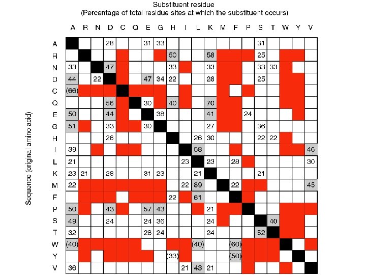
lysine found at 58% of arginine sites Emile Zuckerkandl and Linus Pauling (1965) considered substitution frequencies in 18 globins (myoglobins and hemoglobins from human to lamprey). Black: identity Gray: very conservative substitutions (>40% occurrence) White: fairly conservative substitutions (>21% occurrence) Red: no substitutions observed

PAM 250 log odds scoring matrix that assigns scores and is forgiving of mismatches… (such as +17 for W to W or -5 for W to T)

…and a whole series of scoring matrices such as PAM 10 that are strict and do not tolerate mismatches (such as +13 for W to W or -19 for W to T)

Dayhoff’s 34 protein superfamilies Protein PAMs per 100 million years Ig kappa chain Kappa casein luteinizing hormone b lactalbumin complement component 3 epidermal growth factor proopiomelanocortin pancreatic ribonuclease haptoglobin alpha serum albumin phospholipase A 2, group IB prolactin carbonic anhydrase C Hemoglobin a Hemoglobin b 37 33 30 27 27 26 21 21 20 19 19 17 16 12 12

Dayhoff’s 34 protein superfamilies Protein PAMs per 100 million years Ig kappa chain 37 Kappa casein 33 luteinizing hormone b 30 lactalbumin 27 complement component 3 27 epidermal growth factor 26 proopiomelanocortin 21 pancreatic ribonuclease 21 human (NP_005203) versus mouse (NP_031812) haptoglobin alpha 20 serum albumin 19 phospholipase A 2, group IB 19 prolactin 17 carbonic anhydrase C 16 Hemoglobin a 12 Hemoglobin b 12

Dayhoff’s 34 protein superfamilies Protein PAMs per 100 million years apolipoprotein A-II lysozyme gastrin myoglobin nerve growth factor myelin basic protein thyroid stimulating hormone b parathyroid hormone parvalbumin trypsin insulin calcitonin arginine vasopressin adenylate kinase 1 10 9. 8 8. 9 8. 5 7. 4 7. 3 7. 0 5. 9 4. 4 4. 3 3. 6 3. 2

Dayhoff’s 34 protein superfamilies Protein PAMs per 100 million years triosephosphate isomerase 1 vasoactive intestinal peptide glyceraldehyde phosph. dehydrogease cytochrome c collagen troponin C, skeletal muscle alpha crystallin B chain glucagon glutamate dehydrogenase histone H 2 B, member Q ubiquitin 2. 8 2. 6 2. 2 1. 7 1. 5 1. 2 0. 9 0

Pairwise alignment of human (NP_005203) versus mouse (NP_031812) ubiquitin

Dayhoff’s approach to assigning scores for any two aligned amino acid residues Dayhoff et al. defined the score of two aligned residues i, j as 10 times the log of how likely it is to observe these two residues (based on the empirical observation of how often they are aligned in nature) divided by the background probability of finding these amino acids by chance. This provides a score for each pair of residues.

Dayhoff’s numbers of “accepted point mutations”: what amino acid substitutions occur in proteins? Dayhoff (1978) p. 346.

Multiple sequence alignment of glyceraldehyde 3 -phosphate dehydrogenases: columns of residues may have high or low conservation fly human plant bacterium yeast archaeon GAKKVIISAP GAKRVIISAP GAKKVVMTGP GAKKVVITAP GADKVLISAP SAD. APM. . F SKDNTPM. . F SS. TAPM. . F PKGDEPVKQL VCGVNLDAYK VMGVNHEKYD VVGVNEHTYQ VKGANFDKY. VMGVNEEKYT VYGVNHDEYD PDMKVVSNAS NSLKIISNAS PNMDIVSNAS AGQDIVSNAS SDLKIVSNAS GE. DVVSNAS CTTNCLAPLA CTTNCLAPLA CTTNSITPVA fly human plant bacterium yeast archaeon KVINDNFEIV KVIHDNFGIV KVVHEEFGIL KVINDNFGII KVINDAFGIE KVLDEEFGIN EGLMTTVHAT EGLMTTVHAI EGLMTTVHAT EGLMTTVHSL AGQLTTVHAY TATQKTVDGP TATQKTVDGP TGSQNLMDGP SGKLWRDGRG SMKDWRGGRG SHKDWRGGRT NGKP. RRRRA AAQNIIPAST ALQNIIPAST ASQNIIPSST ASGNIIPSST AAENIIPTST fly human plant bacterium yeast archaeon GAAKAVGKVI GAAKAVGKVL GAAQAATEVL PALNGKLTGM PELNGKLTGM PELQGKLTGM PELEGKLDGM AFRVPTPNVS AFRVPTANVS AFRVPTSNVS AFRVPTPNVS AFRVPTVDVS AIRVPVPNGS VVDLTVRLGK VVDLTCRLEK VVDLTVRLEK VVDLTVKLNK ITEFVVDLDD GASYDEIKAK PAKYDDIKKV GASYEDVKAA AATYEQIKAA ETTYDEIKKV DVTESDVNAA

The relative mutability of amino acids Asn Ser Asp Glu Ala Thr Ile Met Gln Val 134 120 106 102 100 97 96 94 93 74 His Arg Lys Pro Gly Tyr Phe Leu Cys Trp 66 65 56 56 49 41 41 40 20 18

Normalized frequencies of amino acids Gly Ala Leu Lys Ser Val Thr Pro Glu Asp 8. 9% 8. 7% 8. 5% 8. 1% 7. 0% 6. 5% 5. 8% 5. 1% 5. 0% 4. 7% Arg Asn Phe Gln Ile His Cys Tyr Met Trp • blue=6 codons; red=1 codon • These frequencies fi sum to 1 4. 1% 4. 0% 3. 8% 3. 7% 3. 4% 3. 3% 3. 0% 1. 5% 1. 0%

Dayhoff’s numbers of “accepted point mutations”: what amino acid substitutions occur in proteins?

Dayhoff’s PAM 1 mutation probability matrix Original amino acid A Ala R Arg N Asn D Asp C Cys Q Gln E Glu G Gly H His I Ile A 9867 2 9 10 3 8 17 21 2 6 R 1 9913 1 0 1 10 0 0 10 3 N 4 1 9822 36 0 4 6 6 21 3 D 6 0 42 9859 0 6 53 6 4 1 C 1 1 0 0 9973 0 0 0 1 1 Q 3 9 4 5 0 9876 27 1 23 1 E 10 0 7 56 0 35 9865 4 2 3 G 21 1 12 11 1 3 7 9935 1 0 H 1 8 18 3 1 20 1 0 9912 0 I 2 2 3 1 2 0 0 9872 Mutation probability matrix for the evolutionary distance of 1 PAM (i. e. , one Accepted Point Mutation per 100 amino acids). An element of this matrix, [Mij], gives the probability that the amino acid in column j will be replaced by the amino acid in row i after a given evolutionary interval, in this case 1 PAM. Thus, there is a 0. 56% probability that Asp will be replaced by Glu. To simplify the appearance, the elements are shown multiplied by 10, 000

Substitution Matrix A substitution matrix contains values proportional to the probability that amino acid i mutates into amino acid j for all pairs of amino acids. Substitution matrices are constructed by assembling a large and diverse sample of verified pairwise alignments (or multiple sequence alignments) of amino acids. Substitution matrices should reflect the true probabilities of mutations occurring through a period of evolution. The two major types of substitution matrices are PAM and BLOSUM.

PAM matrices: Point-accepted mutations PAM matrices are based on global alignments of closely related proteins. The PAM 1 is the matrix calculated from comparisons of sequences with no more than 1% divergence. At an evolutionary interval of PAM 1, one change has occurred over a length of 100 amino acids. Other PAM matrices are extrapolated from PAM 1. For PAM 250, 250 changes have occurred for two proteins over a length of 100 amino acids. All the PAM data come from closely related proteins (>85% amino acid identity).

Dayhoff’s PAM 0 mutation probability matrix: the rules for extremely slowly evolving proteins Top: original amino acid Side: replacement amino acid

Dayhoff’s PAM 2000 mutation probability matrix: the rules for very distantly related proteins PAM A R N D C Q E G Ala Arg Asn Asp Cys Gln Glu Gly A 8. 7% 8. 7% R 4. 1% 4. 1% N 4. 0% 4. 0% D 4. 7% 4. 7% C 3. 3% 3. 3% Q 3. 8% 3. 8% E 5. 0% 5. 0% G 8. 9% 8. 9% Top: original amino acid Side: replacement amino acid

PAM 250 mutation probability matrix Top: original amino acid Side: replacement amino acid

PAM 250 log odds scoring matrix

Why do we go from a mutation probability matrix to a log odds matrix? • We want a scoring matrix so that when we do a pairwise alignment (or a BLAST search) we know what score to assign to two aligned amino acid residues. • Logarithms are easier to use for a scoring system. They allow us to sum the scores of aligned residues (rather than having to multiply them).

How do we go from a mutation probability matrix to a log odds matrix? • The cells in a log odds matrix consist of an “odds ratio”: the probability that an alignment is authentic the probability that the alignment was random The score S for an alignment of residues a, b is given by: S(a, b) = 10 log 10 (Mab/pb) As an example, for tryptophan, S(trp, trp) = 10 log 10 (0. 55/0. 010) = 17. 4

What do the numbers mean in a log odds matrix? A score of +2 indicates that the amino acid replacement occurs 1. 6 times as frequently as expected by chance. A score of 0 is neutral. A score of – 10 indicates that the correspondence of two amino acids in an alignment that accurately represents homology (evolutionary descent) is one tenth as frequent as the chance alignment of these amino acids.

More conserved Rat versus mouse globin Less conserved Rat versus bacterial globin

two nearly identical proteins two distantly related proteins

BLOSUM Matrices BLOSUM matrices are based on local alignments. BLOSUM stands for blocks substitution matrix. BLOSUM 62 is a matrix calculated from comparisons of sequences with no less than 62% divergence.

62 co l e ps la Percent amino acid identity BLOSUM Matrices 100 30 BLOSUM 62

100 e lla 100 30 e ps 30 62 lla 62 co l la ps co Percent amino acid identity 100 ps e BLOSUM Matrices BLOSUM 80 BLOSUM 62 30 BLOSUM 30

BLOSUM Matrices All BLOSUM matrices are based on observed alignments; they are not extrapolated from comparisons of closely related proteins. The BLOCKS database contains thousands of groups of multiple sequence alignments. BLOSUM 62 is the default matrix in BLAST 2. 0. Though it is tailored for comparisons of moderately distant proteins, it performs well in detecting closer relationships. A search for distant relatives may be more sensitive with a different matrix.

Blosum 62 scoring matrix

PAM matrices: Point-accepted mutations PAM matrices are based on global alignments of closely related proteins. The PAM 1 is the matrix calculated from comparisons of sequences with no more than 1% divergence. At an evolutionary interval of PAM 1, one change has occurred over a length of 100 amino acids. Other PAM matrices are extrapolated from PAM 1. For PAM 250, 250 changes have occurred for two proteins over a length of 100 amino acids. All the PAM data come from closely related proteins (>85% amino acid identity).

Percent identity Two randomly diverging protein sequences change in a negatively exponential fashion “twilight zone” Evolutionary distance in PAMs

Percent identity At PAM 1, two proteins are 99% identical At PAM 10. 7, there are 10 differences per 100 residues At PAM 80, there are 50 differences per 100 residues At PAM 250, there are 80 differences per 100 residues “twilight zone” Differences per 100 residues

PAM: “Accepted point mutation” • Two proteins with 50% identity may have 80 changes per 100 residues. (Why? Because any residue can be subject to back mutations. ) • Proteins with 20% to 25% identity are in the “twilight zone” and may be statistically significantly related. • PAM or “accepted point mutation” refers to the “hits” or matches between two sequences (Dayhoff & Eck, 1968)

Two kinds of sequence alignment: global and local We will first consider the global alignment algorithm of Needleman and Wunsch (1970). We will then explore the local alignment algorithm of Smith and Waterman (1981).

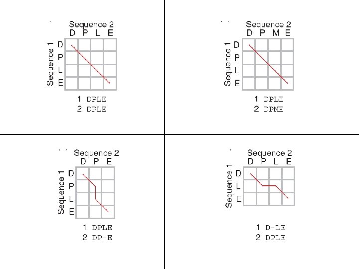
Global alignment with the algorithm of Needleman and Wunsch (1970) • Two sequences can be compared in a matrix along x- and y-axes. • If they are identical, a path along a diagonal can be drawn • Find the optimal subpaths, and add them up to achieve the best score. This involves --adding gaps when needed --allowing for conservative substitutions --choosing a scoring system (simple or complicated) • N-W is guaranteed to find optimal alignment(s)

Three steps to global alignment with the Needleman-Wunsch algorithm [1] set up a matrix [2] score the matrix [3] identify the optimal alignment(s)

Four possible outcomes in aligning two sequences 1 2 [1] identity (stay along a diagonal) [2] mismatch (stay along a diagonal) [3] gap in one sequence (move vertically) [4] gap in the other sequence (move horizontally)

Start Needleman-Wunsch with an identity matrix

Start Needleman-Wunsch with an identity matrix

Fill in the matrix using “dynamic programming”

Fill in the matrix using “dynamic programming”

Fill in the matrix using “dynamic programming”

Fill in the matrix using “dynamic programming”

Fill in the matrix using “dynamic programming”

Fill in the matrix using “dynamic programming”

Fill in the matrix using “dynamic programming”

Traceback to find the optimal (best) pairwise alignment

Needleman-Wunsch: dynamic programming N-W is guaranteed to find optimal alignments, although the algorithm does not search all possible alignments. It is an example of a dynamic programming algorithm: an optimal path (alignment) is identified by incrementally extending optimal subpaths. Thus, a series of decisions is made at each step of the alignment to find the pair of residues with the best score.

Try using needle to implement a Needleman. Wunsch global alignment algorithm to find the optimum alignment (including gaps): http: //www. ebi. ac. uk/emboss/align/

Queries: beta globin (NP_000509) alpha globin (NP_000549)

Global alignment versus local alignment Global alignment (Needleman-Wunsch) extends from one end of each sequence to the other. Local alignment finds optimally matching regions within two sequences (“subsequences”). Local alignment is almost always used for database searches such as BLAST. It is useful to find domains (or limited regions of homology) within sequences. Smith and Waterman (1981) solved the problem of performing optimal local sequence alignment. Other methods (BLAST, FASTA) are faster but less thorough.

Global alignment (top) includes matches ignored by local alignment (bottom) 15% identity 30% identity NP_824492, NP_337032

How the Smith-Waterman algorithm works Set up a matrix between two proteins (size m+1, n+1) No values in the scoring matrix can be negative! S > 0 The score in each cell is the maximum of four values: [1] s(i-1, j-1) + the new score at [i, j] (a match or mismatch) [2] s(i, j-1) – gap penalty [3] s(i-1, j) – gap penalty [4] zero

Smith-Waterman algorithm allows the alignment of subsets of sequences

Try using SSEARCH to perform a rigorous Smith. Waterman local alignment: http: //fasta. bioch. virginia. edu/

Queries: beta globin (NP_000509) alpha globin (NP_000549)

Rapid, heuristic versions of Smith-Waterman: FASTA and BLAST Smith-Waterman is very rigorous and it is guaranteed to find an optimal alignment. But Smith-Waterman is slow. It requires computer space and time proportional to the product of the two sequences being aligned (or the product of a query against an entire database). Gotoh (1982) and Myers and Miller (1988) improved the algorithms so both global and local alignment require less time and space. FASTA and BLAST provide rapid alternatives to S-W.

Pairwise alignments with dot plots: graphical displays of relatedness with NCBI’s BLAST [1] Compare human cytoglobin (NP_599030, length 190 amino acids) with itself. The output includes a dot plot. The data points showing amino acid identities appear as a diagonal line. [2] Compare cytoglobin with a globin from the snail Biomphalaria glabrata (accession CAJ 44466, length 2, 148 amino acids. See lots of repeated regions!

Pairwise alignments with dot plots: cytoglobin versus itself yields a straight line

Pairwise alignments with dot plots: cytoglobin versus itself (but with 15 amino acids deleted from one copy)

Pairwise alignments with dot plots: cytoglobin versus a snail globin