Sequence Alignment and Phylogenetic Analysis Evolution Sequence Alignment

Sequence Alignment and Phylogenetic Analysis

Evolution

Sequence Alignment AGGCTATCACCTGACCTCCAGGCCGATGCCC TAGCTATCACGACCGCGGTCGATTTGCCCGAC -AGGCTATCACCTGACCTCCAGGCCGA--TGCCC--TAG-CTATCAC--GACCGC--GGTCGATTTGCCCGAC Definition Given two strings x = x 1 x 2. . . x. M, y = y 1 y 2…y. N, an alignment is an assignment of gaps to positions 0, …, N in x, and 0, …, N in y, so as to line up each letter in one sequence with either a letter, or a gap in the other sequence

A E G H W A 5 -1 0 -2 -3 E -1 6 -3 0 -3 H -2 0 -2 10 -3 P -1 -1 -2 -2 -4 W -3 -3 15 Example H E A G A W G H E E 0 -8 -16 -24 -32 -40 -48 -56 -64 -72 -80 P -8 -2 -9 -17 -25 -33 -42 -49 -57 -65 -73 A -16 W -24 H -32 E -40 A -48 E -56 4

A E G H W A 5 -1 0 -2 -3 E -1 6 -3 0 -3 H -2 0 -2 10 -3 P -1 -1 -2 -2 -4 W -3 -3 15 H E A G A W G H E E 0 -8 -16 -24 -32 -40 -48 -56 -64 -72 -80 P -8 -2 -9 -17 -25 -33 -42 -49 -57 -65 -73 A -16 -10 -3 -4 -12 -20 -28 -36 -44 -52 -60 W -24 -18 -11 -6 -7 -15 -5 -13 -21 -29 -37 H -32 -14 -18 -13 -8 -9 -13 -7 -3 -11 -19 E -40 -22 -8 -16 -9 -12 -15 -7 3 -5 A -48 -30 -16 -3 -11 -12 -15 -5 2 E -56 -38 -24 -11 -6 -12 -14 -15 -12 -9 1 5

The Blosum 50 Scoring Matrix

Multiple Alignment

Example

Clustal. W • Popular multiple alignment tool today • ‘W’ stands for ‘weighted’ (different parts of alignment are weighted differently). • Three-step process 1. ) Construct pairwise alignments 2. ) Build Guide Tree 3. ) Progressive Alignment guided by the tree

Step 1: Pairwise Alignment

Step 3: Progressive Alignment • Start by aligning the two most similar sequences • Following the guide tree, add in the next sequences, aligning to the existing alignment • Insert gaps as necessary

Some Guidelines for Choosing the Right Sequences

Gathering Sequences with BLAST • The most convenient way to select your sequences is to use a BLAST server • Some BLAST servers are integrated with multiple-alignment methods: • www. expasy. ch (protein only) • srs. ebi. ac. uk (DNA/protein) • npsa-pbil. ibcp. fr

Selecting a Method • Many alternative methods exist for MSAs • Most of them use the progressive algorithm • They all are approximate methods • None is guaranteed to deliver the best alignments • All existing methods have pros and cons • Clustal. W is the most popular (21, 000 citations) • T-Coffee and Prob. Cons are more accurate but slower • MUSCLE is very fast, ideal for very large datasets

Clustal. W • www. ebi. ac. uk/clustalw • pir. georgetown. edu/pirwww/search/multia ln. shtml • www. ddbj. nig. ac. jp/search/clustalw-e. html

Tcoffee • • TCOFFEE: www. tcoffee. org CORE: evaluate MSA MCOFFEE: run many and combine EXPRESSO: with structural information

Running Many Methods at Once • MCOFFEE is a a meta-method • It runs all the individual MSA methods • It gathers all the produced MSAs • It combines the MSAs into a single MSA • MCOFFEE is more accurate than any individual method • Its color output lets you estimate the reliability of your MSA • MCOFFEE is available on www. tcoffee. org

Editing and Publishing Alignments

Alignments and Formats • Many alternative formats exist for MSAs • One format does not always have a clear advantage over another • Changing formats is possible • Annotation information can sometimes be lost in a format change • Not all formats contain the same information • The annotation may change • Reformatting may cause the loss of annotation information

The Most Common Sequence Formats

Interleaved and Non-interleaved ü The MSF Format Interleaved ü The FASTA Format Non-interleaved

Choosing Your Format • When choosing a format, ask yourself four questions: • Is it supported by the programs I need to use ? • Can my collaborators use it? • Can it support all of my annotation ? • Is it easy to read and manipulate ?

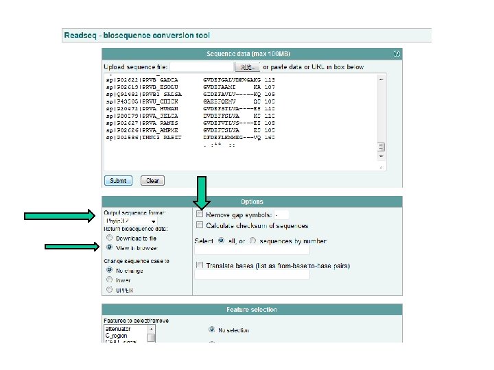
Converting Formats • Don’t re-compute your MSA if it is not in the right format • Convert your file using one of the online conversion tools • The 3 most popular reformatting utilities: • Fmtseq • RESDSEQ • Seq. Check The most complete Very popular and robust Can clean FASTA sequences

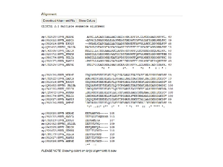
CLUSTAL 2. 1 multiple sequence alignment sp|P 02620|PRVB_MERME sp|P 02622|PRVB_GADCA sp|P 02619|PRVB_ESOLU sp|Q 91482|PRVB 1_SALSA sp|P 43305|PRVU_CHICK sp|P 20472|PRVA_HUMAN sp|P 80079|PRVA_FELCA sp|P 02627|PRVA_RANES sp|P 02626|PRVA_AMPME sp|P 02586|TNNC 2_RABIT An Alignment -----------------------AFAGI 5 -----------------------AFKGI 5 -----------------------SFAGL 5 ----------------------MACAHL 6 ----------------------MSLTDI 6 --------------------------------------------MSMTDL 6 -----------------------PMTDL 5 -----------------------SMTDV 5 MTDQQAEARSYLSEEMIAEFKAAFDMFDADGGGDISVKELGTVMRMLGQT 50 sp|P 02620|PRVB_MERME LADADITAALAACKAEGS--FKHGEFFTKIG------LKGKSAADIKKVF 47 sp|P 02622|PRVB_GADCA LSNADIKAAEAACFKEGS--FDEDGFYAKVG------LDAFSADELKKLF 47 sp|P 02619|PRVB_ESOLU -KDADVAAALAACSAADS--FKHKEFFAKVG------LASKSLDDVKKAF 46 sp|Q 91482|PRVB 1_SALSA CKEADIKTALEACKAADT--FSFKTFFHTIG------FASKSADDVKKAF 48 sp|P 43305|PRVU_CHICK LSPSDIAAALRDCQAPDS--FSPKKFFQISG------MSKKSSSQLKEIF 48 sp|P 20472|PRVA_HUMAN LNAEDIKKAVGAFSATDS--FDHKKFFQMVG------LKKKSADDVKKVF 48 sp|P 80079|PRVA_FELCA LGAEDIKKAVEAFTAVDS--FDYKKFFQMVG------LKKKSPDDIKKVF 48 sp|P 02627|PRVA_RANES LAAGDISKAVSAFAAPES--FNHKKFFELCG------LKSKSKEIMQKVF 47 sp|P 02626|PRVA_AMPME IPEADINKAIHAFKAGEA--FDFKKFVHLLG------LNKRSPADVTKAF 47 sp|P 02586|TNNC 2_RABIT PTKEELDAIIEEVDEDGSGTIDFEEFLVMMVRQMKEDAKGKSEEELAECF 100 : : . * * : : * sp|P 02620|PRVB_MERME sp|P 02622|PRVB_GADCA sp|P 02619|PRVB_ESOLU sp|Q 91482|PRVB 1_SALSA sp|P 43305|PRVU_CHICK sp|P 20472|PRVA_HUMAN sp|P 80079|PRVA_FELCA sp|P 02627|PRVA_RANES sp|P 02626|PRVA_AMPME sp|P 02586|TNNC 2_RABIT : *. : : ** GIIDQDKSDFVEEDELKLFLQNFSAGARALTDAETATFLKAGDSDGDGKI 97 KIADEDKEGFIEEDELKLFLIAFAADLRALTDAETKAFLKAGDSDGDGKI 97 YVIDQDKSGFIEEDELKLFLQNFSPSARALTDAETKAFLADGDKDGDGMI 96 KVIDQDASGFIEVEELKLFLQNFCPKARELTDAETKAFLKAGDADGDGMI 98 RILDNDQSGFIEEDELKYFLQRFECGARVLTASETKTFLAAADHDGDGKI 98 HMLDKDKSGFIEEDELGFILKGFSPDARDLSAKETKMLMAAGDKDGDGKI 98 HILDKDKSGFIEEDELGFILKGFYPDARDLSVKETKMLMAAGDKDGDGKI 98 HVLDQDQSGFIEKEELCLILKGFTPEGRSLSDKETTALLAAGDKDGDGKI 97 HILDKDRSGYIEEEELQLILKGFSKEGRELTDKETKDLLIKGDKDGDGKI 97 RIFDRNADGYIDAEELAEIFR---ASGEHVTDEEIESLMKDGDKNNDGRI 147 : : * : : . ** * sp|P 02620|PRVB_MERME sp|P 02622|PRVB_GADCA sp|P 02619|PRVB_ESOLU sp|Q 91482|PRVB 1_SALSA sp|P 43305|PRVU_CHICK sp|P 20472|PRVA_HUMAN sp|P 80079|PRVA_FELCA sp|P 02627|PRVA_RANES sp|P 02626|PRVA_AMPME sp|P 02586|TNNC 2_RABIT. : ** : : GVEEFAAMV-----KG 108 GVDEFGALVDKWGAKG 113 GVDEFAAMI-----KA 107 GIDEFAVLV-----KQ 109 GAEEFQEMV-----QS 109 GVDEFSTLVA----ES 110 DVDEFFSLVA----KS 110 GVDEFVTLVS----ES 109 GVDEFTSLVA----ES 109 DFDEFLKMMEG---VQ 160

READSEQ • http: //www. ebi. ac. uk/cgi-bin/readseq. cgi

Different Formats (PHYLIP)

PHYLIP (no gap)

Different Formats (MSF)

Converting Formats Can Be Dangerous • Format conversion can result in data loss • After converting your file, you must make sure your data is still intact • The following slide shows the most common losses that occur during conversion

Potential Information Loss When Converting MSAs

Editing your MSA • If your MSA looks bad. . . • Don’t torture the online server • Edit the MSA yourself locally • Never, ever (ever) use a standard word processor • Always use a dedicated MSA editor • The most popular online tool is Jalview • You can get it at www. jalview. org

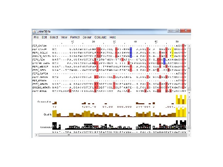
With Jalview You Can. . . • • • Modify your MSA Remove some of the redundant sequences Insert/remove gaps Shift portions of the MSA Modify the alignment of a sub-group of sequences • Recompute some portions of your alignment

Click a sequence to select

Drag to select columns

Some Special Features of Jalview • • Computation of a consensus sequence Computation of a phylogenetic tree Removal of the redundancy Applying any color scheme to your MSA

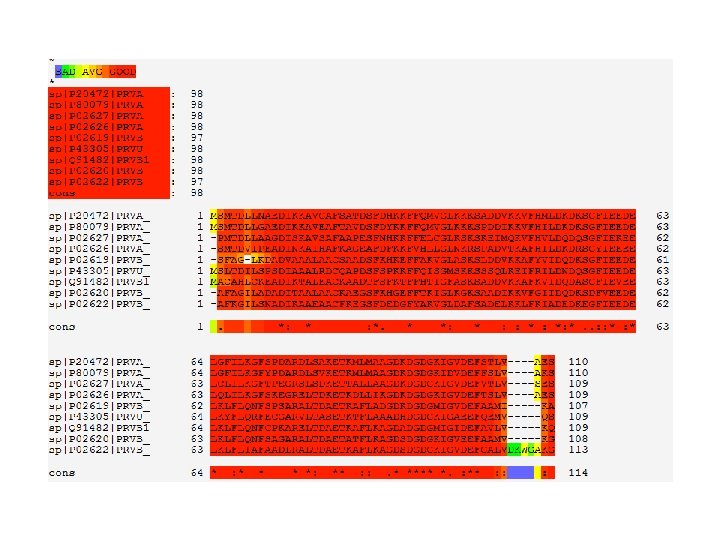
Preparing Your MSA for Publication • MSAs in publications usually come with shaded colors • You can improve your MSAs using online tools like Boxshade • Boxshade will shade your MSA according to its degree of conservation

MSA => LOGO Graph • • A LOGO graph summarizes an MSA Tall letters indicate highly conserved positions Short letters indicate poorly conserved positions LOGO graphs are ideal for identifying conserved patterns • weblogo. berkeley. edu/

Going Farther • Your imagination is the limit when it comes to making MSAs nice- looking and informative • Four very popular and easy-to-install MSA editors: • CINEMA • Seaview • Belvu • Kalignview • Boxshade is the simplest shading tool • If you need heavier capabilities, try Espript • Available at espript. ibpc. fr

Molecular Evolution and Phylogenetic Reconstruction

Early Evolutionary Studies • Anatomical features were the dominant criteria used to derive evolutionary relationships between species since Darwin till early 1960 s • The evolutionary relationships derived from these relatively subjective observations were often inconclusive. Some of them were later proved incorrect

Evolution and DNA Analysis: the Giant Panda Riddle • For roughly 100 years scientists were unable to figure out which family the giant panda belongs to • Giant pandas look like bears but have features that are unusual for bears and typical for raccoons, e. g. , they do not hibernate • In 1985, Steven O’Brien and colleagues solved the giant panda classification problem using DNA sequences and algorithms

Evolutionary Tree of Bears and Raccoons

Evolutionary Trees: DNA-based Approach • 50 years ago: Emile Zuckerkandl and Linus Pauling brought reconstructing evolutionary relationships with DNA into the spotlight • In the first few years after Zuckerkandl and Pauling proposed using DNA for evolutionary studies, the possibility of reconstructing evolutionary trees by DNA analysis was hotly debated • Now it is a dominant approach to study evolution.

Who are closer?

Human-Chimpanzee Split?

Chimpanzee-Gorilla Split?

Three-way Split?

Out of Africa Hypothesis • Around the time the giant panda riddle was solved, a DNA-based reconstruction of the human evolutionary tree led to the Out of Africa Hypothesis that claims our most ancient ancestor lived in Africa roughly 200, 000 years ago

Human Evolutionary Tree (cont’d) http: //www. mun. ca/biology/scarr/Out_of_Africa 2. htm

The Origin of Humans: ”Out of Africa” vs Multiregional Hypothesis Out of Africa: Multiregional: • Humans evolved in the last two Africa ~150, 000 years million years as a single species. ago Independent appearance of modern • Humans migrated out traits in different areas of Africa, replacing other shumanoids • Humans migrated out of Africa around the globe mixing with other humanoids on the • There is no direct way descendence from Neanderthals • There is a genetic continuity from Neanderthals to humans

mt. DNA analysis supports “Out of Africa” Hypothesis • African origin of humans inferred from: • African population was the most diverse (sub-populations had more time to diverge) • The evolutionary tree separated one group of Africans from a group containing all five populations. • Tree was rooted on branch between groups of greatest difference.

Evolutionary Tree of Humans: (microsatellites) Neighbor joining tree for 14 human populations genotyped with 30 microsatellite loci. •

Human Migration Out of Africa 1. Yorubans 2. Western Pygmies 3. Eastern Pygmies 4. Hadza 5. !Kung 1 2 3 4 5 http: //www. becominghuman. org

Two Neanderthal Discoveries Feldhofer, Germany Mezmaiskaya, Caucasus Distance: 2500 km

Two Neanderthal Discoveries • Is there a connection between Neanderthals and today’s Europeans? • If humans did not evolve from Neanderthals, whom did we evolve from?

Multiregional Hypothesis? • May predict some genetic continuity from the Neanderthals through to the Cro. Magnons up to today’s Europeans • Can explain the occurrence of varying regional characteristics

Sequencing Neanderthal’s mt. DNA • mt. DNA from the bone of Neanderthal is used because it is up to 1, 000 x more abundant than nuclear DNA • DNA decay overtime and only a small amount of ancient DNA can be recovered (upper limit: 100, 000 years) • PCR of mt. DNA (fragments are too short, human DNA may mixed in)

Neanderthals vs Humans: surprisingly large divergence • AMH vs Neanderthal: • 22 substitutions and 6 indels in 357 bp region • AMH vs AMH • only 8 substitutions

Evolutionary Trees How are these trees built from DNA sequences? • leaves represent existing species • internal vertices represent ancestors • root represents the oldest evolutionary ancestor

Reading Your Tree • There’s a lot of vocabulary in a tree • Nodes correspond to common ancestors • The root is the oldest ancestor • Often artificial • Only meaningful with a good outgroup • Trees can be un-rooted • Branch lengths are only meaningful when the tree is scaled • Cladograms are often scaled • Phenograms are usualy unscaled

Rooted and Unrooted Trees In the unrooted tree the position of the root (“oldest ancestor”) is unknown. Otherwise, they are like rooted trees

Type of Trees (Cladogram)

Type of Trees (Phylogram)

3 Ways to Use Your Tree • Finding the closest relative of your organism • Usually done with a tree based on the ribosomal RNA • Discovering the function of a gene • Finding the orthologues of your gene • Finding the origin of your gene • Finding whether your gene comes from another species

Evolutionary Rate • Normal mutation rate is 1 in 10 -8 nucleotides • Normal Polymorphic Variance. Approximately 1 in every 1000 nucleotides • This is the background on which evolutionary • changes are analyzed.

Orthology and Paralogy • Orthologous genes 直系（垂直）同源和旁系（平行）同源 • Separated by speciation • Often have the same function • Paralogous genes • Separated by duplications • Can have different functions • In the graph: • A is paralogous with B • A 1 is orthologous with A 2

Working on the Right Data • Garbage in garbage out • The quality of your tree depends on the quality of the data • Your first task is to assemble a very accurate MSA

DNA or Proteins • Most phylogenetic methods work on Proteins and DNA sequences • If possible, always compute a multiple-sequence alignment on the protein sequences • Translate the sequences if the DNA is coding • Align the sequences • Thread the DNA sequences back onto the protein MSA with coot. embl. de/pal 2 nal • If your DNA sequences are coding and have more than 70% identity. . . • Compute the tree on the DNA multiple-sequence alignment • If your DNA sequences are coding and have less than 70% identity. . . • Compute the tree on the protein multiple-sequence alignment

Which Sequences ? • Orthologous sequences • Produce a species tree • Show the considered species have diverged • Paralogous sequences • Produce a gene tree • Show the evolution of a protein family

Establishing Orthology • Establishing orthology is very complicated • It is common practice to establish orthology using the best reciprocal BLAST • • A is a gene of Genome X B is a gene of Genome Y BLAST (Gene A against Genome X) = B BLAST (Gene B against Genome Y) = A • A is B’s best friend and B is A’s best friend… • Phylogeny purists dislike this method

Creating the Perfect Dataset

Building the Right MSA • Your MSA should have as few gaps as possible. Most time should remove columns with gaps. • Some variability but not too much! • Some conservation but not too much!

Building the Right Tree • There are three types of tree-reconstruction methods • Distance-based methods • Statistical methods • Parsimony methods • Statistical methods are the most accurate • Maximum likelihood of success • Bayesian methods • Statistical methods take more time • Limited to small datasets

Distance-based method • Compute a distance matrix • Try to fit the matrix to a tree • Fast but may not be very accurate

Distances in Trees • Edges may have weights reflecting: • Number of mutations on evolutionary path from one species to another • Time estimate for evolution of one species into another • In a tree T, we often compute dij(T) - the length of a path between leaves i and j dij(T) – tree distance between i and j

Distance in Trees: an Exampe j i d 1, 4 = 12 + 13 + 14 + 17 + 12 = 68

Distance Matrix • Given n species, we can compute the n x n distance matrix Dij • Dij may be defined as the edit distance between a gene in species i and species j, where the gene of interest is sequenced for all n species. Dij – edit distance between i and j

Edit Distance vs. Tree Distance • Given n species, we can compute the n x n distance matrix Dij • Dij may be defined as the edit distance between a gene in species i and species j, where the gene of interest is sequenced for all n species. Dij – edit distance between i and j • Note the difference with dij(T) – tree distance between i and j

Compute a Distance Matrix Evolutionary Distance - number of substitutions per 100 amino acids (for proteins) or nucleotides (for DNA) A C T G T A G G A A T C G C A A T G A A A G A A T C G C 3 observed changes A C T G T A G G A A T C G C A C T G C A G G A A T A G C A A T G A A A G A A T C G C 6 actual changes

Edit Distance vs Tree Distance j i d 1, 4 = 12 + 13 + 14 + 17 + 12 = 68 D 1, 4 may be smaller than 68, as some changes may not be observed

Fitting Distance Matrix • Given n species, we can compute the n x n distance matrix Dij • Evolution of these genes is described by a tree that we don’t know. • We need an algorithm to construct a tree that best fits the distance matrix Dij

Fitting Distance Matrix Lengths of path in an (unknown) tree T • Fitting means Dij = dij(T) Edit distance between species (known)

Reconstructing a 3 Leaved Tree • Tree reconstruction for any 3 x 3 matrix is straightforward • We have 3 leaves i, j, k and a center vertex c Observe: dic + djc = Dij dic + dkc = Dik djc + dkc = Djk

Reconstructing a 3 Leaved Tree (cont’d) dic + djc = Dij + dic + dkc = Dik 2 dic + djc + dkc = Dij + Dik 2 dic + Djk = Dij + Dik dic = (Dij + Dik – Djk)/2 Similarly, djc = (Dij + Djk – Dik)/2 dkc = (Dki + Dkj – Dij)/2

Trees with > 3 Leaves • An tree with n leaves has 2 n-3 edges • This means fitting a given tree to a distance matrix D requires solving a system of “n choose 2” equations with 2 n-3 variables • This is not always possible to solve for n > 3

Additive Distance Matrices Matrix D is ADDITIVE if there exists a tree T with dij(T) = Dij NON-ADDITIVE otherwise

Distance Based Phylogeny Problem • Goal: Reconstruct an evolutionary tree from a distance matrix • Input: n x n distance matrix Dij • Output: weighted tree T with n leaves fitting D • If D is additive, this problem has a solution and there is a simple algorithm to solve it

Using Neighboring Leaves to Construct the Tree • Find neighboring leaves i and j with parent k • Remove the rows and columns of i and j • Add a new row and column corresponding to k, where the distance from k to any other leaf m can be computed as: Dkm = (Dim + Djm – Dij)/2 Compress i and j into k, iterate algorithm for rest of tree

Finding Neighboring Leaves • To find neighboring leaves we simply select a pair of closest leaves.

Finding Neighboring Leaves • To find neighboring leaves we simply select a pair of closest leaves. WRONG

Finding Neighboring Leaves • Closest leaves aren’t necessarily neighbors • i and j are neighbors, but (dij = 13) > (djk = 12) • Finding a pair of neighboring leaves is a nontrivial problem!

Neighbor Joining Algorithm • In 1987 Naruya Saitou and Masatoshi Nei developed a neighbor joining algorithm for phylogenetic tree reconstruction • Finds a pair of leaves that are close to each other but far from other leaves: implicitly finds a pair of neighboring leaves • Advantages: works well for additive and other nonadditive matrices, it does not have the flawed molecular clock assumption