Chapter 3 Pairwise Sequence Alignment Jonathan Pevsner Ph

Chapter 3: Pairwise Sequence Alignment Jonathan Pevsner, Ph. D. pevsner@kennedykrieger. org Bioinformatics and Functional Genomics (Wiley-Liss, 3 rd edition, 2015) You may use this Power. Point for teaching

Learning objectives Upon completion of this material , you should be able to: • define homology as well as orthologs and paralogs; • explain how PAM (accepted point mutation) matrices are derived; • contrast the utility of PAM and BLOSUM scoring matrices; • define dynamic programming and explain how global (Needleman–Wunsch) and local (Smith–Waterman) pairwise alignments are performed; and • perform pairwise alignment of protein or DNA sequences at the NCBI website.

Outline Introduction Protein alignment: often more informative than DNA alignment Definitions: homology, similarity, identity Gaps Pairwise alignment, homology, and evolution of life Scor. Ing matrices Dayhoff model: 7 steps Pairwise alignment and limits of detection: the “twilight zone” Al. Ignment algorithms: global and local Global sequence alignment: algorithm of Needleman and Wunsch Local sequence alignment: Smith and Waterman algorithm Rapid, heuristic versions of Smith–Waterman: FASTA and BLAST Basic Local Alignment Search Tool (BLAST) Pairwise alignment with dotplots The statistical significance of pairwise alignments Statistical significance of global alignments

Pairwise sequence alignment is the most fundamental operation of bioinformatics • It is used to decide if two proteins (or genes) are related structurally or functionally • It is used to identify domains or motifs that are shared between proteins • It is the basis of BLAST searching • It is used in the analysis of genomes B&FG 3 e Page 69

Sequence alignment: protein sequences can be more informative than DNA • protein is more informative (20 vs 4 characters); many amino acids share related biophysical properties • codons are degenerate: changes in the third position often do not alter the amino acid that is specified • protein sequences offer a longer “look-back” time Example: --searching for plant globins using human beta globin DNA yields no matches; --searching for plant globins using human beta globin protein yields many matches B&FG 3 e Page 70

Pairwise alignment: DNA sequences can be more informative than protein • Many times, DNA alignments are appropriate --to study noncoding regions of DNA (e. g. introns or intergenic regions) --to study DNA polymorphisms --genome sequencing relies on DNA analysis B&FG 3 e Page 70

Definition: pairwise alignment Pairwise alignment The process of lining up two sequences to achieve maximal levels of identity (and conservation, in the case of amino acid sequences) for the purpose of assessing the degree of similarity and the possibility of homology. B&FG 3 e Page 70

Definitions: identity, similarity, conservation Homology Similarity attributed to descent from a common ancestor. Identity The extent to which two (nucleotide or amino acid) sequences are invariant. Similarity The extent to which nucleotide or protein sequences are related. It is based upon identity plus conservation. Conservation B&FG 3 e Page 70 Changes at a specific position of an amino acid or (less commonly, DNA) sequence that preserve the physico-chemical properties of the original residue.

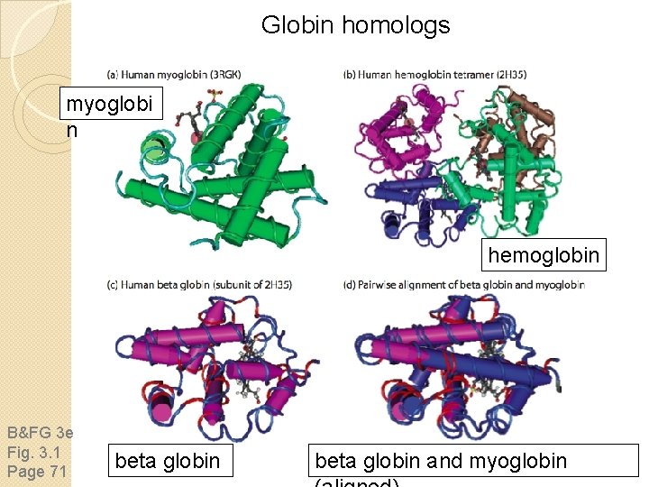
Globin homologs myoglobi n hemoglobin B&FG 3 e Fig. 3. 1 Page 71 beta globin and myoglobin

Outline Introduction Protein alignment: often more informative than DNA alignment Definitions: homology, similarity, identity Gaps Pairwise alignment, homology, and evolution of life Scor. Ing matrices Dayhoff model: 7 steps Pairwise alignment and limits of detection: the “twilight zone” Al. Ignment algorithms: global and local Global sequence alignment: algorithm of Needleman and Wunsch Local sequence alignment: Smith and Waterman algorithm Rapid, heuristic versions of Smith–Waterman: FASTA and BLAST Basic Local Alignment Search Tool (BLAST) Pairwise alignment with dotplots The statistical significance of pairwise alignments Statistical significance of global alignments

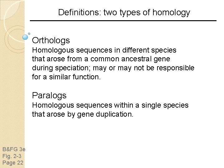
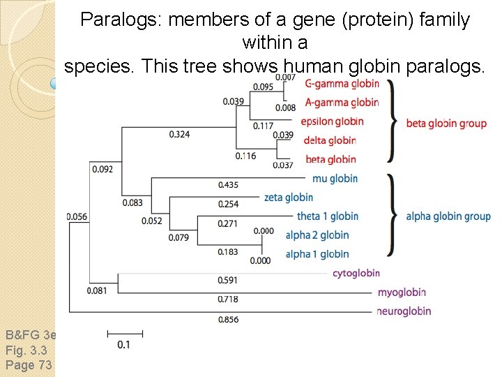
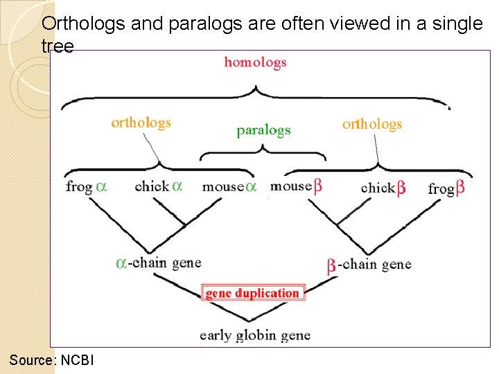
Definitions: two types of homology Orthologs Homologous sequences in different species that arose from a common ancestral gene during speciation; may or may not be responsible for a similar function. Paralogs Homologous sequences within a single species that arose by gene duplication. B&FG 3 e Fig. 2 -3 Page 22

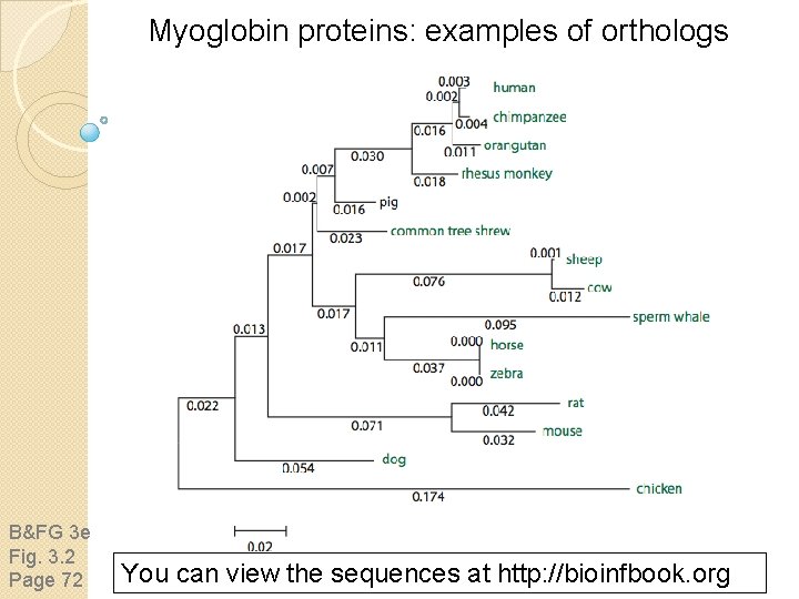
Myoglobin proteins: examples of orthologs B&FG 3 e Fig. 3. 2 Page 72 You can view the sequences at http: //bioinfbook. org

Paralogs: members of a gene (protein) family within a species. This tree shows human globin paralogs. B&FG 3 e Fig. 3. 3 Page 73

Orthologs and paralogs are often viewed in a single tree Source: NCBI

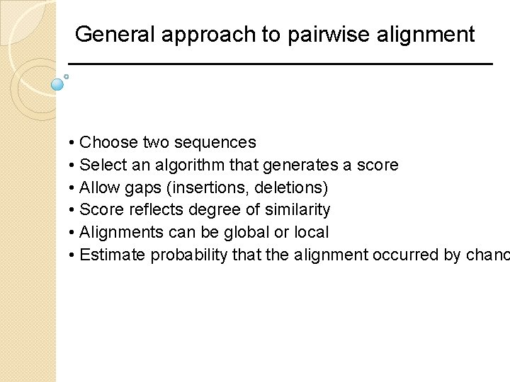
General approach to pairwise alignment • Choose two sequences • Select an algorithm that generates a score • Allow gaps (insertions, deletions) • Score reflects degree of similarity • Alignments can be global or local • Estimate probability that the alignment occurred by chanc

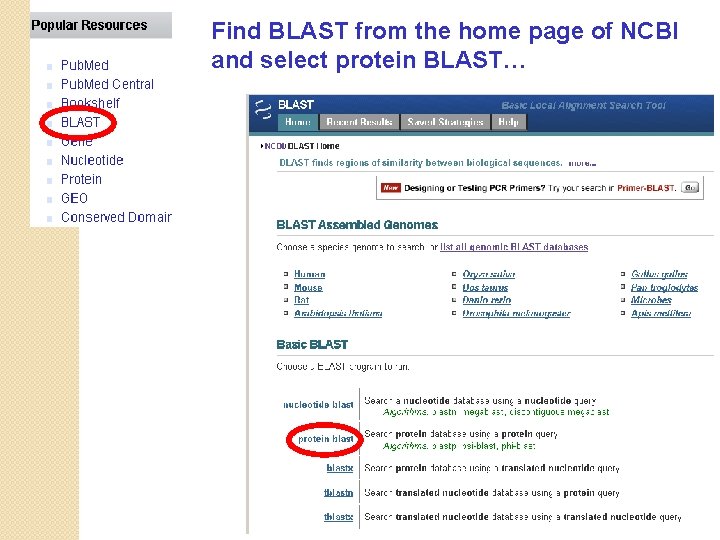
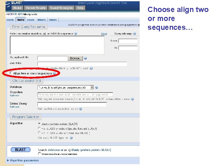
Find BLAST from the home page of NCBI and select protein BLAST…

Choose align two or more sequences…

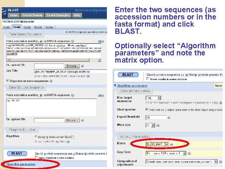
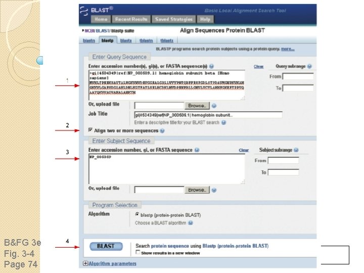
Enter the two sequences (as accession numbers or in the fasta format) and click BLAST. Optionally select “Algorithm parameters” and note the matrix option.

sequence B&FG 3 e Fig. 3 -4 Page 74 Year

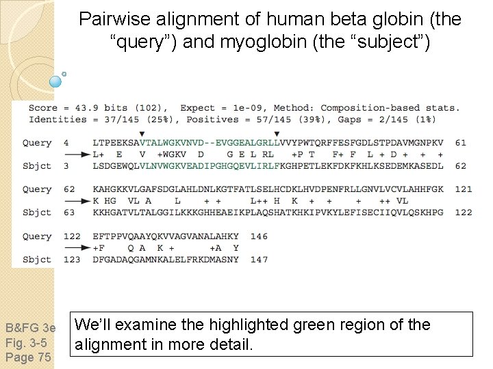
Pairwise alignment of human beta globin (the “query”) and myoglobin (the “subject”) B&FG 3 e Fig. 3 -5 Page 75 We’ll examine the highlighted green region of the alignment in more detail.

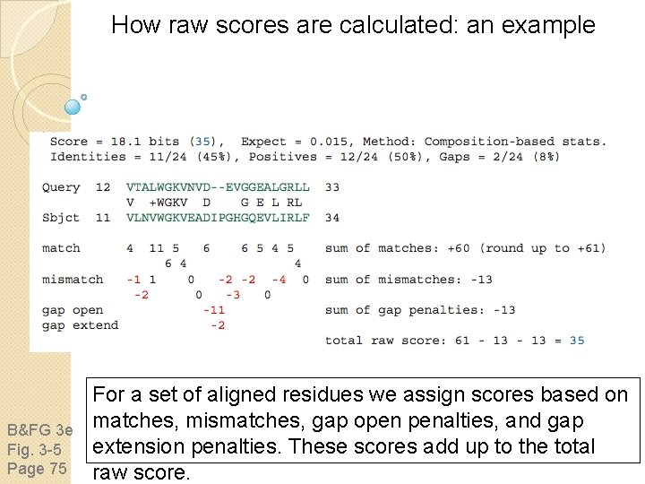
How raw scores are calculated: an example B&FG 3 e Fig. 3 -5 Page 75 For a set of aligned residues we assign scores based on matches, mismatches, gap open penalties, and gap extension penalties. These scores add up to the total raw score.

B&FG 3 e Box 3 -6 Page 83

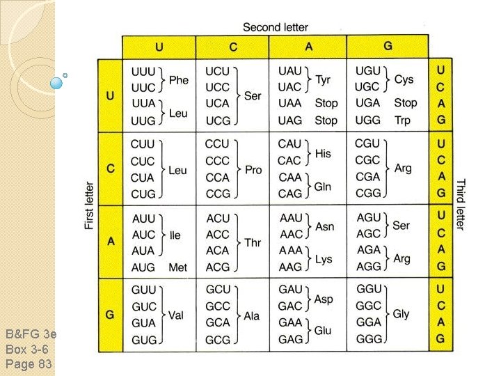
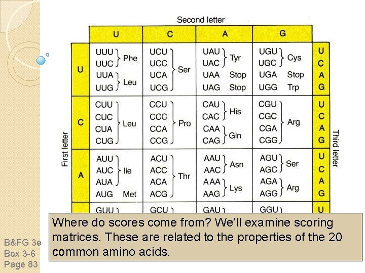
B&FG 3 e Box 3 -6 Page 83 Where do scores come from? We’ll examine scoring matrices. These are related to the properties of the 20 common amino acids.

Outline Introduction Protein alignment: often more informative than DNA alignment Definitions: homology, similarity, identity Gaps Pairwise alignment, homology, and evolution of life Scor. Ing matrices Dayhoff model: 7 steps Pairwise alignment and limits of detection: the “twilight zone” Al. Ignment algorithms: global and local Global sequence alignment: algorithm of Needleman and Wunsch Local sequence alignment: Smith and Waterman algorithm Rapid, heuristic versions of Smith–Waterman: FASTA and BLAST Basic Local Alignment Search Tool (BLAST) Pairwise alignment with dotplots The statistical significance of pairwise alignments Statistical significance of global alignments

Gaps • Positions at which a letter is paired with a null are called gaps. • Gap scores are typically negative. • Since a single mutational event may cause the insertion or deletion of more than one residue, the presence of a gap is ascribed more significance than the length of the gap. Thus there are separate penalties for gap creation and gap extension. • In BLAST, it is rarely necessary to change gap

Outline Introduction Protein alignment: often more informative than DNA alignment Definitions: homology, similarity, identity Gaps Pairwise alignment, homology, and evolution of life Scor. Ing matrices Dayhoff model: 7 steps Pairwise alignment and limits of detection: the “twilight zone” Al. Ignment algorithms: global and local Global sequence alignment: algorithm of Needleman and Wunsch Local sequence alignment: Smith and Waterman algorithm Rapid, heuristic versions of Smith–Waterman: FASTA and BLAST Basic Local Alignment Search Tool (BLAST) Pairwise alignment with dotplots The statistical significance of pairwise alignments Statistical significance of global alignments

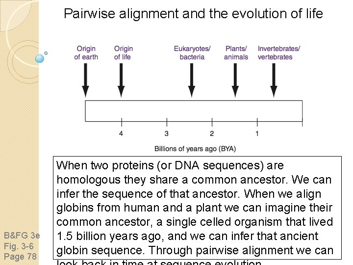
Pairwise alignment and the evolution of life B&FG 3 e Fig. 3 -6 Page 78 When two proteins (or DNA sequences) are homologous they share a common ancestor. We can infer the sequence of that ancestor. When we align globins from human and a plant we can imagine their common ancestor, a single celled organism that lived 1. 5 billion years ago, and we can infer that ancient globin sequence. Through pairwise alignment we can

Outline Introduction Protein alignment: often more informative than DNA alignment Definitions: homology, similarity, identity Gaps Pairwise alignment, homology, and evolution of life Scoring matrices Dayhoff model: 7 steps Pairwise alignment and limits of detection: the “twilight zone” Alignment algorithms: global and local Global sequence alignment: algorithm of Needleman and Wunsch Local sequence alignment: Smith and Waterman algorithm Rapid, heuristic versions of Smith–Waterman: FASTA and BLAST Basic Local Alignment Search Tool (BLAST) Pairwise alignment with dotplots The statistical significance of pairwise alignments Statistical significance of global alignments

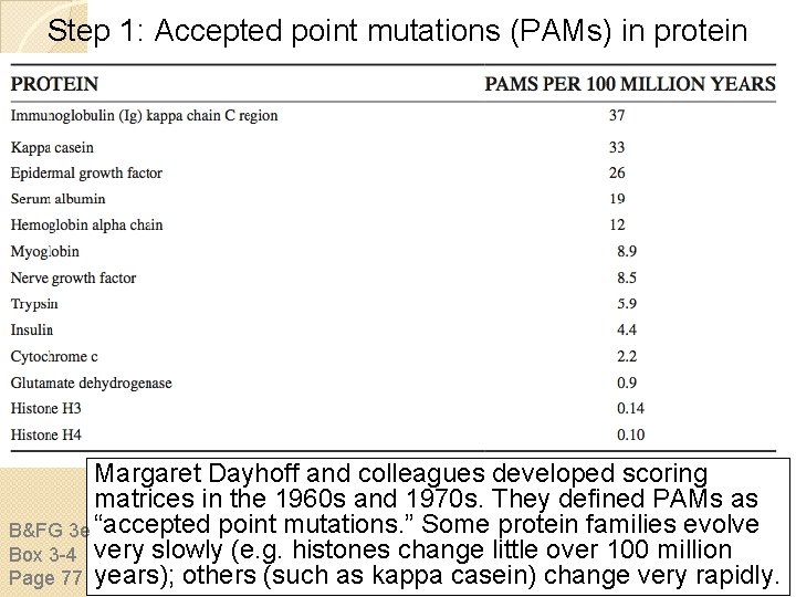
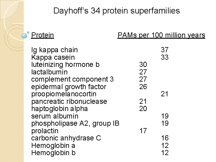
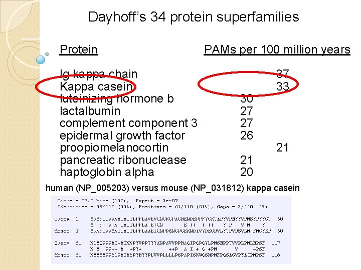
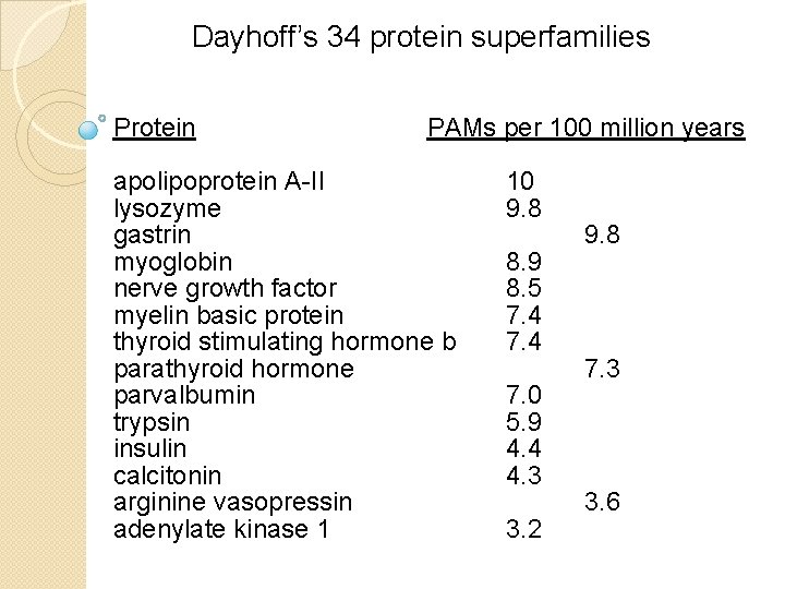
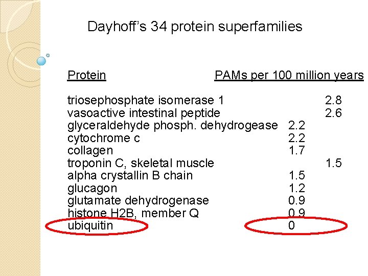
Step 1: Accepted point mutations (PAMs) in protein families Margaret Dayhoff and colleagues developed scoring matrices in the 1960 s and 1970 s. They defined PAMs as B&FG 3 e “accepted point mutations. ” Some protein families evolve Box 3 -4 very slowly (e. g. histones change little over 100 million Page 77 years); others (such as kappa casein) change very rapidly.

Dayhoff’s 34 protein superfamilies Protein PAMs per 100 million years Ig kappa chain Kappa casein luteinizing hormone b lactalbumin complement component 3 epidermal growth factor proopiomelanocortin pancreatic ribonuclease haptoglobin alpha serum albumin phospholipase A 2, group IB prolactin carbonic anhydrase C Hemoglobin a Hemoglobin b 30 27 27 26 21 20 17 37 33 21 19 19 16 12 12

Dayhoff’s 34 protein superfamilies Protein PAMs per 100 million years Ig kappa chain 37 Kappa casein 33 luteinizing hormone b 30 lactalbumin 27 complement component 3 27 epidermal growth factor 26 proopiomelanocortin 21 pancreatic ribonuclease 21 haptoglobin alpha 20 serum albumin 19 human (NP_005203) versus mouse (NP_031812) kappa casein phospholipase A 2, group IB 19 prolactin 17 carbonic anhydrase C 16 Hemoglobin a 12 Hemoglobin b 12

Dayhoff’s 34 protein superfamilies Protein PAMs per 100 million years apolipoprotein A-II lysozyme gastrin myoglobin nerve growth factor myelin basic protein thyroid stimulating hormone b parathyroid hormone parvalbumin trypsin insulin calcitonin arginine vasopressin adenylate kinase 1 10 9. 8 8. 9 8. 5 7. 4 7. 0 5. 9 4. 4 4. 3 3. 2 9. 8 7. 3 3. 6

Dayhoff’s 34 protein superfamilies Protein PAMs per 100 million years triosephosphate isomerase 1 vasoactive intestinal peptide glyceraldehyde phosph. dehydrogease cytochrome c collagen troponin C, skeletal muscle alpha crystallin B chain glucagon glutamate dehydrogenase histone H 2 B, member Q ubiquitin 2. 2 1. 7 1. 5 1. 2 0. 9 0 2. 8 2. 6 1. 5

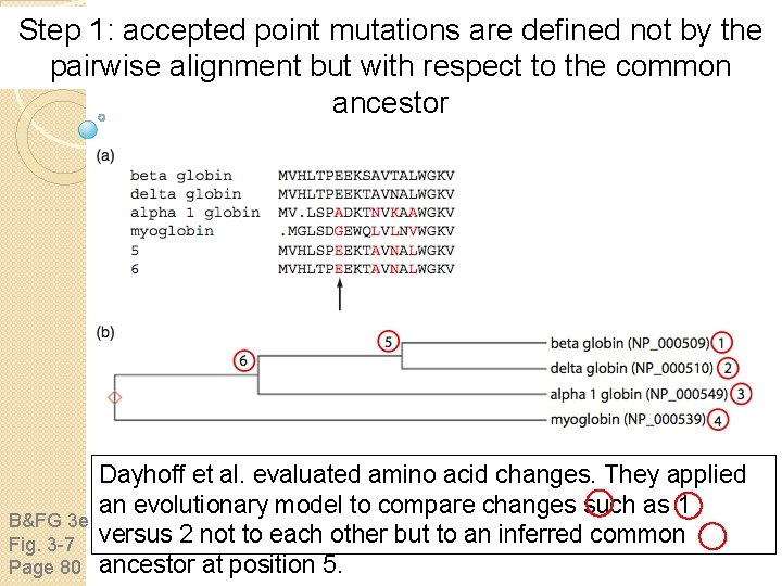
Step 1: accepted point mutations are defined not by the pairwise alignment but with respect to the common ancestor B&FG 3 e Fig. 3 -7 Page 80 Dayhoff et al. evaluated amino acid changes. They applied an evolutionary model to compare changes such as 1 versus 2 not to each other but to an inferred common ancestor at position 5.

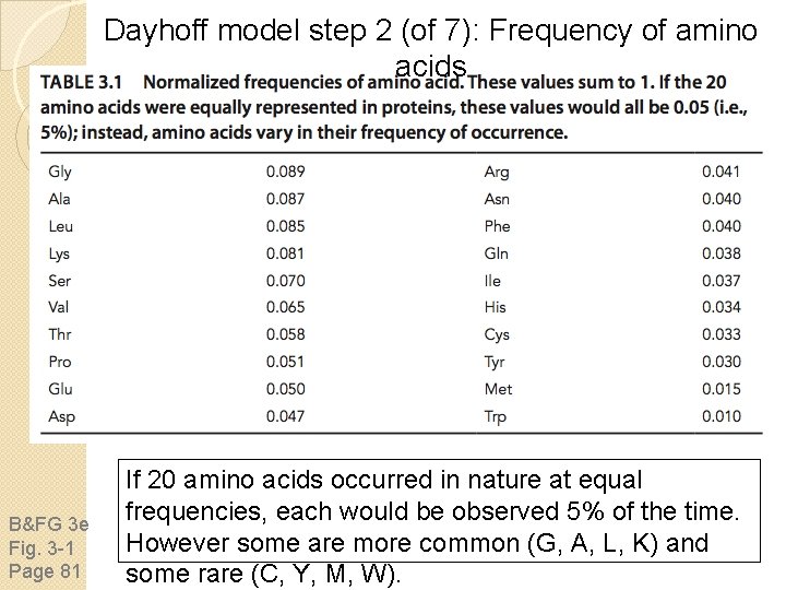
Dayhoff model step 2 (of 7): Frequency of amino acids B&FG 3 e Fig. 3 -1 Page 81 If 20 amino acids occurred in nature at equal frequencies, each would be observed 5% of the time. However some are more common (G, A, L, K) and some rare (C, Y, M, W).

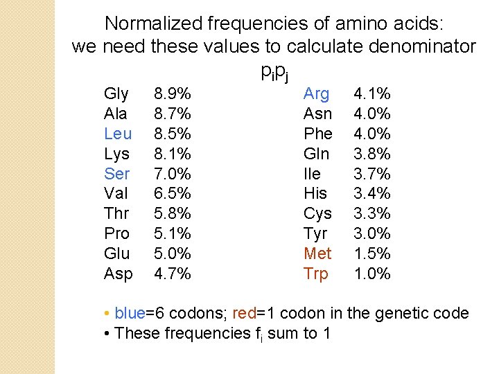
Normalized frequencies of amino acids: we need these values to calculate denominator p ip j Gly Ala Leu Lys Ser Val Thr Pro Glu Asp 8. 9% 8. 7% 8. 5% 8. 1% 7. 0% 6. 5% 5. 8% 5. 1% 5. 0% 4. 7% Arg Asn Phe Gln Ile His Cys Tyr Met Trp 4. 1% 4. 0% 3. 8% 3. 7% 3. 4% 3. 3% 3. 0% 1. 5% 1. 0% • blue=6 codons; red=1 codon in the genetic code • These frequencies fi sum to 1

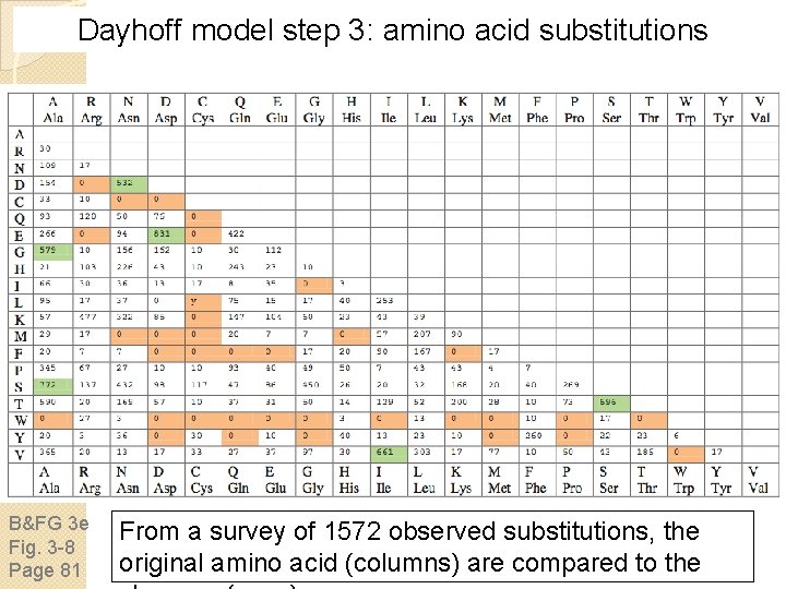
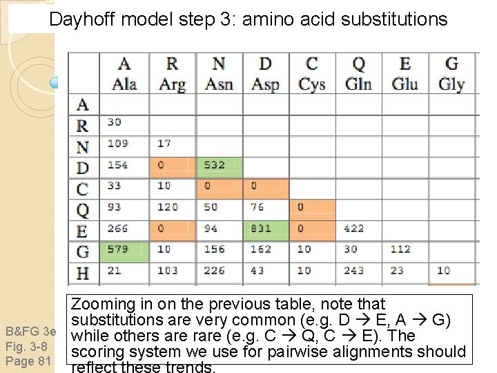
Dayhoff model step 3: amino acid substitutions B&FG 3 e Fig. 3 -8 Page 81 From a survey of 1572 observed substitutions, the original amino acid (columns) are compared to the

Dayhoff model step 3: amino acid substitutions B&FG 3 e Fig. 3 -8 Page 81 Zooming in on the previous table, note that substitutions are very common (e. g. D E, A G) while others are rare (e. g. C Q, C E). The scoring system we use for pairwise alignments should

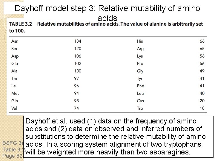
Dayhoff model step 3: Relative mutability of amino acids Dayhoff et al. used (1) data on the frequency of amino acids and (2) data on observed and inferred numbers of substitutions to determine the relative mutability of amino B&FG 3 e acids. In a scoring system alignment of two tryptophans Table 3 -2 will be weighted more heavily than two asparagines. Page 82

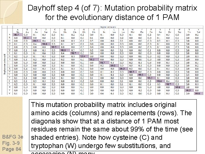
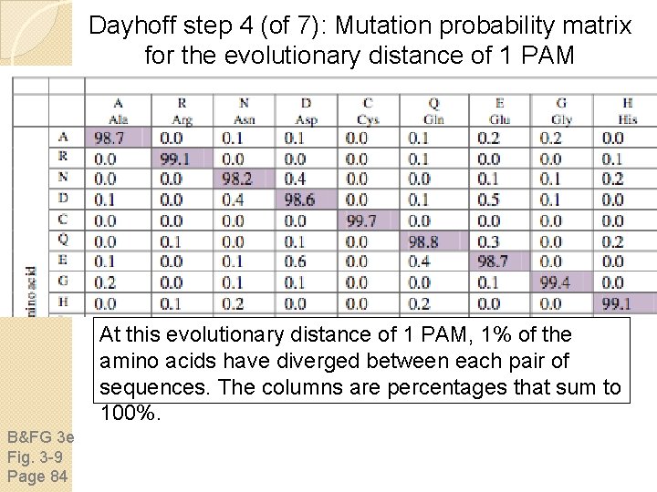
Dayhoff step 4 (of 7): Mutation probability matrix for the evolutionary distance of 1 PAM B&FG 3 e Fig. 3 -9 Page 84 This mutation probability matrix includes original amino acids (columns) and replacements (rows). The diagonals show that at a distance of 1 PAM most residues remain the same about 99% of the time (see shaded entries). Note how cysteine (C) and tryptophan (W) undergo few substitutions, and

Substitution Matrix A substitution matrix contains values proportional to the probability that amino acid i mutates into amino acid j for all pairs of amino acids. Substitution matrices are constructed by assembling a large and diverse sample of verified pairwise alignments (or multiple sequence alignments) of amino acids. Substitution matrices should reflect the true probabilities of mutations occurring through a period of evolution. The two major types of substitution matrices are PAM and BLOSUM.

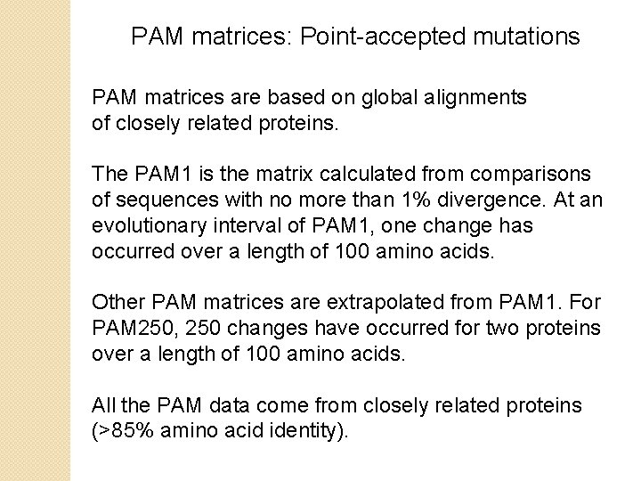
PAM matrices: Point-accepted mutations PAM matrices are based on global alignments of closely related proteins. The PAM 1 is the matrix calculated from comparisons of sequences with no more than 1% divergence. At an evolutionary interval of PAM 1, one change has occurred over a length of 100 amino acids. Other PAM matrices are extrapolated from PAM 1. For PAM 250, 250 changes have occurred for two proteins over a length of 100 amino acids. All the PAM data come from closely related proteins (>85% amino acid identity).

Dayhoff step 4 (of 7): Mutation probability matrix for the evolutionary distance of 1 PAM At this evolutionary distance of 1 PAM, 1% of the amino acids have diverged between each pair of sequences. The columns are percentages that sum to 100%. B&FG 3 e Fig. 3 -9 Page 84

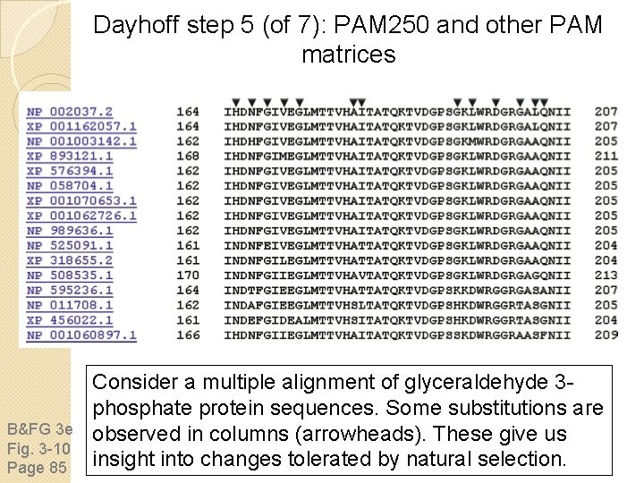
Dayhoff step 5 (of 7): PAM 250 and other PAM matrices B&FG 3 e Fig. 3 -10 Page 85 Consider a multiple alignment of glyceraldehyde 3 phosphate protein sequences. Some substitutions are observed in columns (arrowheads). These give us insight into changes tolerated by natural selection.

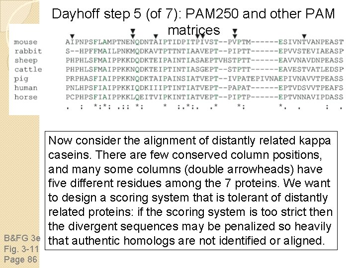
Dayhoff step 5 (of 7): PAM 250 and other PAM matrices B&FG 3 e Fig. 3 -11 Page 86 Now consider the alignment of distantly related kappa caseins. There are few conserved column positions, and many some columns (double arrowheads) have five different residues among the 7 proteins. We want to design a scoring system that is tolerant of distantly related proteins: if the scoring system is too strict then the divergent sequences may be penalized so heavily that authentic homologs are not identified or aligned.

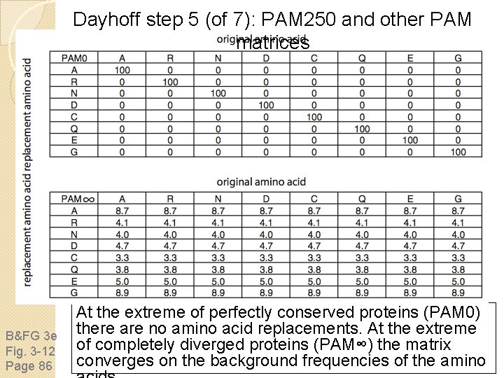
Dayhoff step 5 (of 7): PAM 250 and other PAM matrices B&FG 3 e Fig. 3 -12 Page 86 At the extreme of perfectly conserved proteins (PAM 0) there are no amino acid replacements. At the extreme of completely diverged proteins (PAM∞) the matrix converges on the background frequencies of the amino

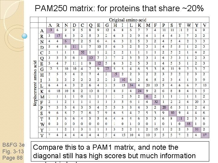
PAM 250 matrix: for proteins that share ~20% identity B&FG 3 e Fig. 3 -13 Page 88 Compare this to a PAM 1 matrix, and note the diagonal still has high scores but much information

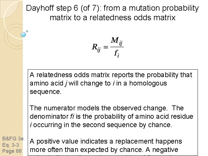
Dayhoff step 6 (of 7): from a mutation probability matrix to a relatedness odds matrix A relatedness odds matrix reports the probability that amino acid j will change to i in a homologous sequence. The numerator models the observed change. The denominator fi is the probability of amino acid residue i occurring in the second sequence by chance. B&FG 3 e Eq. 3 -3 Page 88 A positive value indicates a replacement happens more often than expected by chance. A negative

Why do we go from a mutation probability matrix to a log odds matrix? • We want a scoring matrix so that when we do a pairwise alignment (or a BLAST search) we know what score to assign to two aligned amino acid residues. • Logarithms are easier to use for a scoring system. They allow us to sum the scores of aligned residues (rather than having to multiply them).

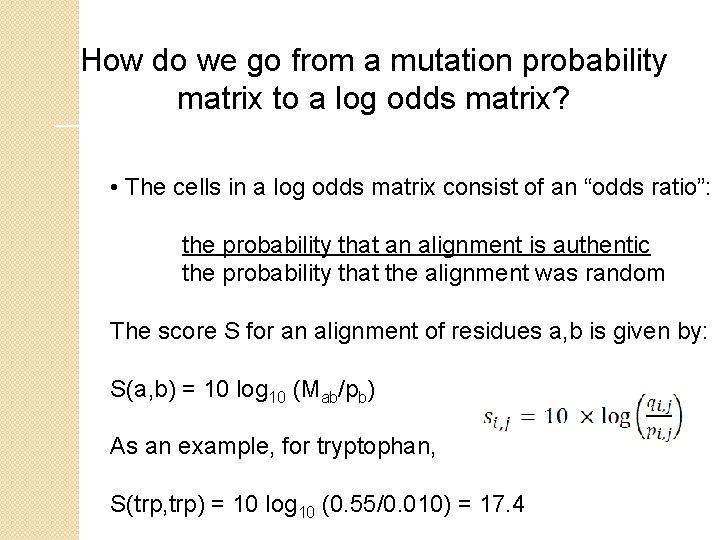
How do we go from a mutation probability matrix to a log odds matrix? • The cells in a log odds matrix consist of an “odds ratio”: the probability that an alignment is authentic the probability that the alignment was random The score S for an alignment of residues a, b is given by: S(a, b) = 10 log 10 (Mab/pb) As an example, for tryptophan, S(trp, trp) = 10 log 10 (0. 55/0. 010) = 17. 4

What do the numbers mean in a log odds matrix? A score of +2 indicates that the amino acid replacement occurs 1. 6 times as frequently as expected by chance. A score of 0 is neutral. A score of – 10 indicates that the correspondence of two amino acids in an alignment that accurately represents homology (evolutionary descent) is one tenth as frequent as the chance alignment of these amino acids.

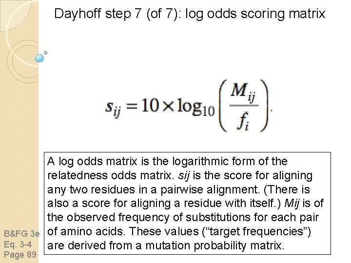
Dayhoff step 7 (of 7): log odds scoring matrix B&FG 3 e Eq. 3 -4 Page 89 A log odds matrix is the logarithmic form of the relatedness odds matrix. sij is the score for aligning any two residues in a pairwise alignment. (There is also a score for aligning a residue with itself. ) Mij is of the observed frequency of substitutions for each pair of amino acids. These values (“target frequencies”) are derived from a mutation probability matrix.

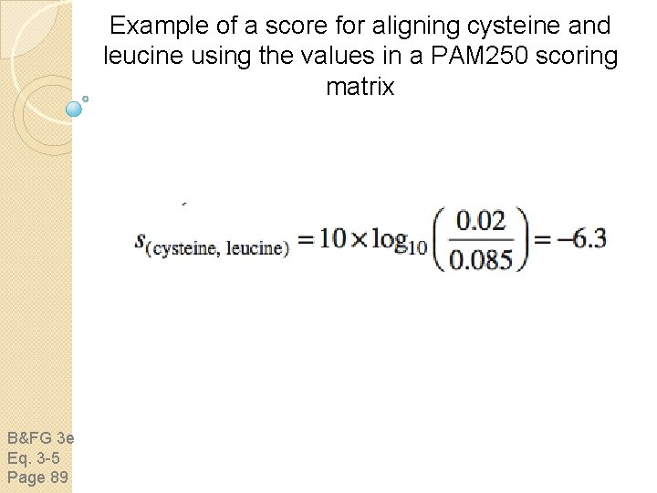
Example of a score for aligning cysteine and leucine using the values in a PAM 250 scoring matrix B&FG 3 e Eq. 3 -5 Page 89

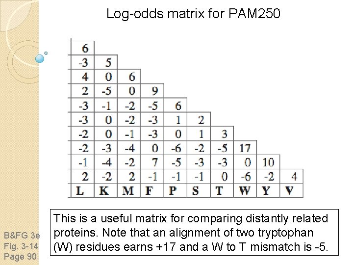
Log-odds matrix for PAM 250 B&FG 3 e Fig. 3 -14 Page 90 This is a useful matrix for comparing distantly related proteins. Note that an alignment of two tryptophan (W) residues earns +17 and a W to T mismatch is -5.

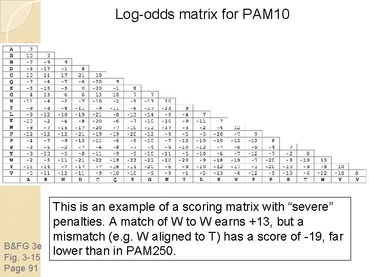
Log-odds matrix for PAM 10 B&FG 3 e Fig. 3 -15 Page 91 This is an example of a scoring matrix with “severe” penalties. A match of W to W earns +13, but a mismatch (e. g. W aligned to T) has a score of -19, far lower than in PAM 250.

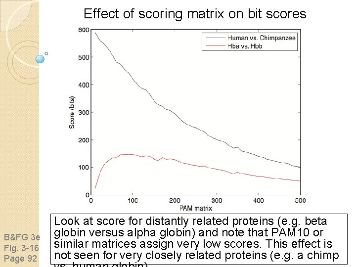
Effect of scoring matrix on bit scores B&FG 3 e Fig. 3 -16 Page 92 Look at score for distantly related proteins (e. g. beta globin versus alpha globin) and note that PAM 10 or similar matrices assign very low scores. This effect is not seen for very closely related proteins (e. g. a chimp

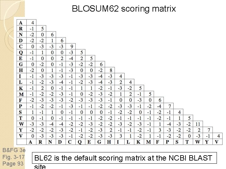
BLOSUM 62 scoring matrix B&FG 3 e Fig. 3 -17 Page 93 BL 62 is the default scoring matrix at the NCBI BLAST

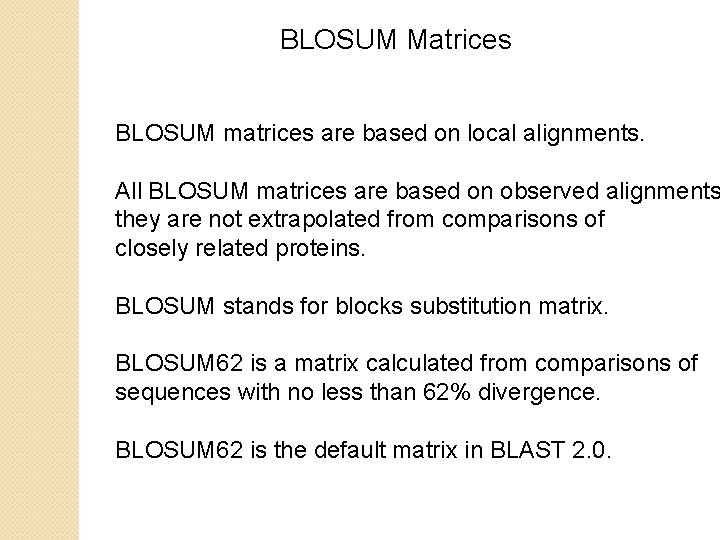
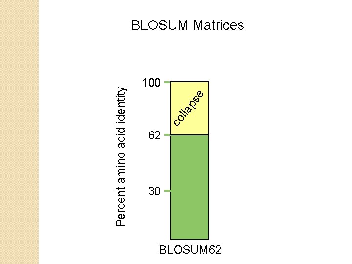
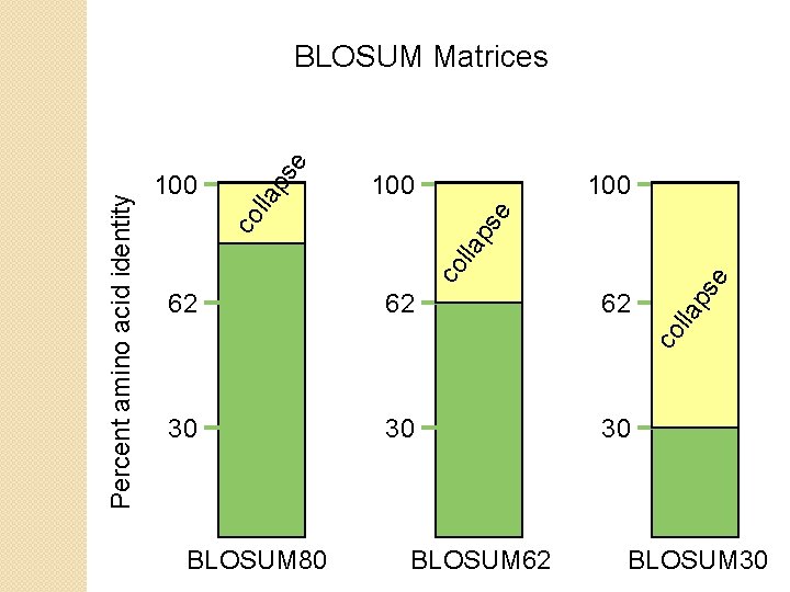
BLOSUM Matrices BLOSUM matrices are based on local alignments. All BLOSUM matrices are based on observed alignments they are not extrapolated from comparisons of closely related proteins. BLOSUM stands for blocks substitution matrix. BLOSUM 62 is a matrix calculated from comparisons of sequences with no less than 62% divergence. BLOSUM 62 is the default matrix in BLAST 2. 0.

e ps lla co Percent amino acid identity BLOSUM Matrices 100 62 30 BLOSUM 62

100 e e ps lla 100 62 30 30 30 lla 62 co 62 ps e co lla ps co Percent amino acid identity BLOSUM Matrices BLOSUM 80 BLOSUM 62 BLOSUM 30

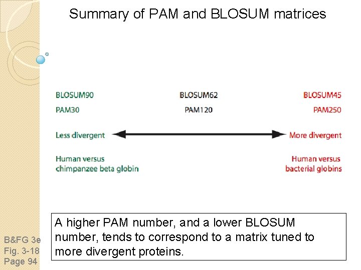
Summary of PAM and BLOSUM matrices B&FG 3 e Fig. 3 -18 Page 94 A higher PAM number, and a lower BLOSUM number, tends to correspond to a matrix tuned to more divergent proteins.

Outline Introduction Protein alignment: often more informative than DNA alignment Definitions: homology, similarity, identity Gaps Pairwise alignment, homology, and evolution of life Scoring matrices Dayhoff model: 7 steps Pairwise alignment and limits of detection: the “twilight zone” Alignment algorithms: global and local Global sequence alignment: algorithm of Needleman and Wunsch Local sequence alignment: Smith and Waterman algorithm Rapid, heuristic versions of Smith–Waterman: FASTA and BLAST Basic Local Alignment Search Tool (BLAST) Pairwise alignment with dotplots The statistical significance of pairwise alignments Statistical significance of global alignments

PAM matrices: Point-accepted mutations PAM matrices are based on global alignments of closely related proteins. The PAM 1 is the matrix calculated from comparisons of sequences with no more than 1% divergence. At an evolutionary interval of PAM 1, one change has occurred over a length of 100 amino acids. Other PAM matrices are extrapolated from PAM 1. For PAM 250, 250 changes have occurred for two proteins over a length of 100 amino acids. All the PAM data come from closely related proteins (>85% amino acid identity).

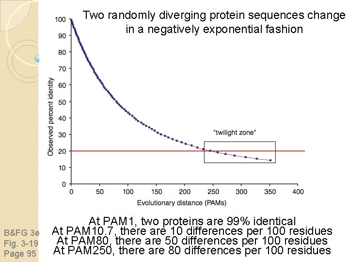
Two randomly diverging protein sequences change in a negatively exponential fashion B&FG 3 e Fig. 3 -19 Page 95 At PAM 1, two proteins are 99% identical At PAM 10. 7, there are 10 differences per 100 residues At PAM 80, there are 50 differences per 100 residues At PAM 250, there are 80 differences per 100 residues

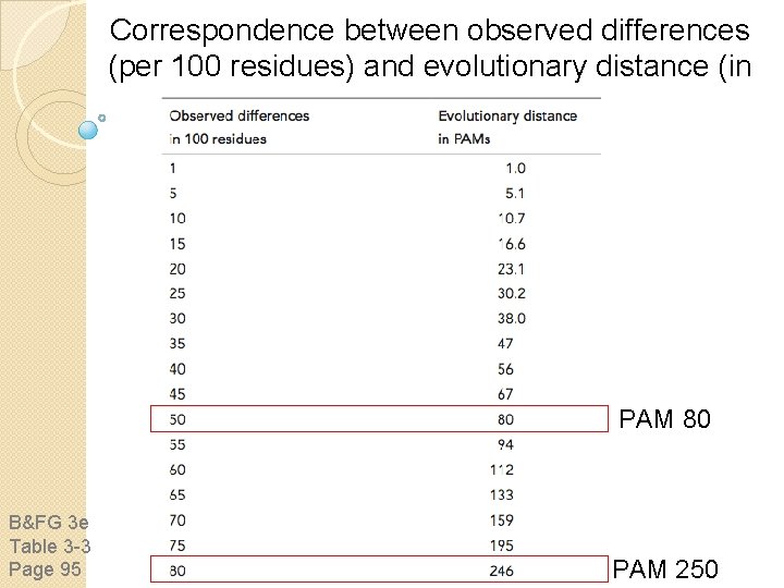
Correspondence between observed differences (per 100 residues) and evolutionary distance (in PAMs) PAM 80 B&FG 3 e Table 3 -3 Page 95 PAM 250

Outline Introduction Protein alignment: often more informative than DNA alignment Definitions: homology, similarity, identity Gaps Pairwise alignment, homology, and evolution of life Scoring matrices Dayhoff model: 7 steps Pairwise alignment and limits of detection: the “twilight zone” Alignment algorithms: global and local Global sequence alignment: algorithm of Needleman and Wunsch Local sequence alignment: Smith and Waterman algorithm Rapid, heuristic versions of Smith–Waterman: FASTA and BLAST Basic Local Alignment Search Tool (BLAST) Pairwise alignment with dotplots The statistical significance of pairwise alignments Statistical significance of global alignments

Two kinds of sequence alignment: global and local We will first consider the global alignment algorithm of Needleman and Wunsch (1970). We will then explore the local alignment algorithm of Smith and Waterman (1981). Finally, we will consider BLAST, a heuristic version of Smith-Waterman.

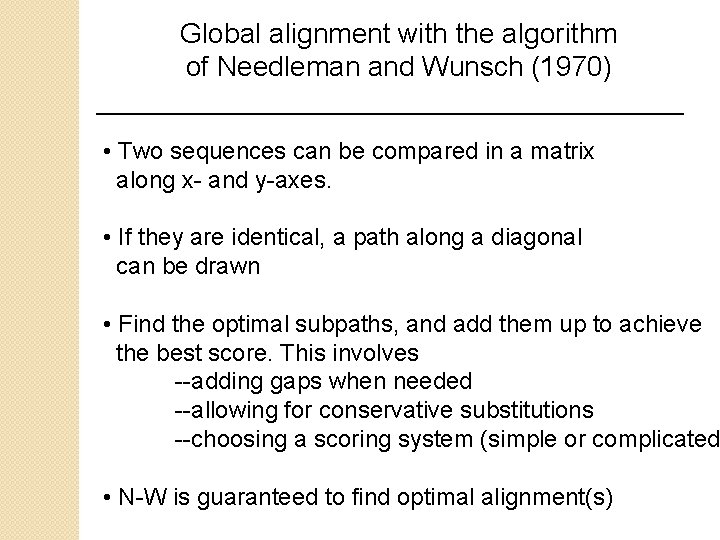
Global alignment with the algorithm of Needleman and Wunsch (1970) • Two sequences can be compared in a matrix along x- and y-axes. • If they are identical, a path along a diagonal can be drawn • Find the optimal subpaths, and add them up to achieve the best score. This involves --adding gaps when needed --allowing for conservative substitutions --choosing a scoring system (simple or complicated • N-W is guaranteed to find optimal alignment(s)

Three steps to global alignment with the Needleman-Wunsch algorithm [1] set up a matrix [2] score the matrix [3] identify the optimal alignment(s)

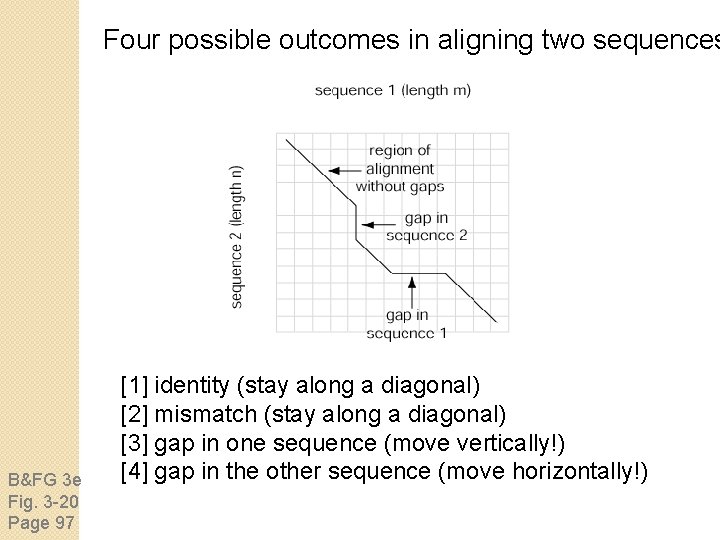
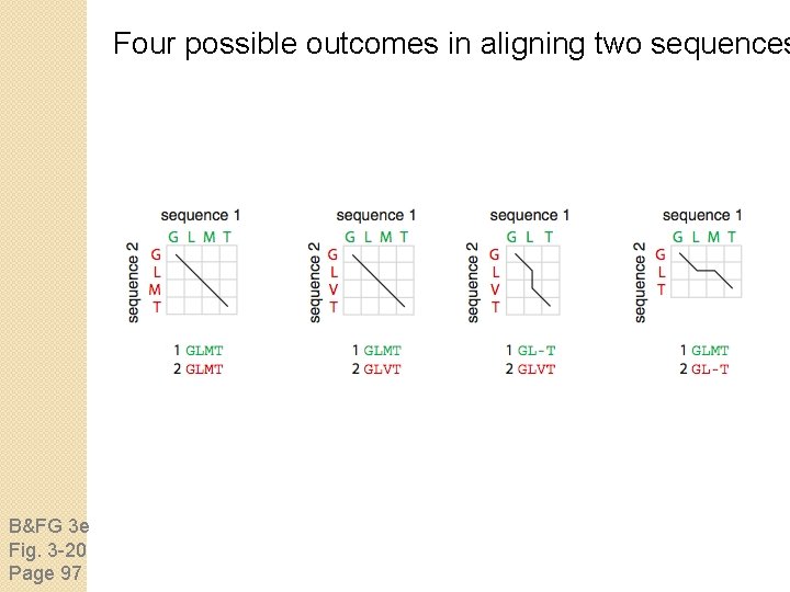
Four possible outcomes in aligning two sequences B&FG 3 e Fig. 3 -20 Page 97 [1] identity (stay along a diagonal) [2] mismatch (stay along a diagonal) [3] gap in one sequence (move vertically!) [4] gap in the other sequence (move horizontally!)

Four possible outcomes in aligning two sequences B&FG 3 e Fig. 3 -20 Page 97

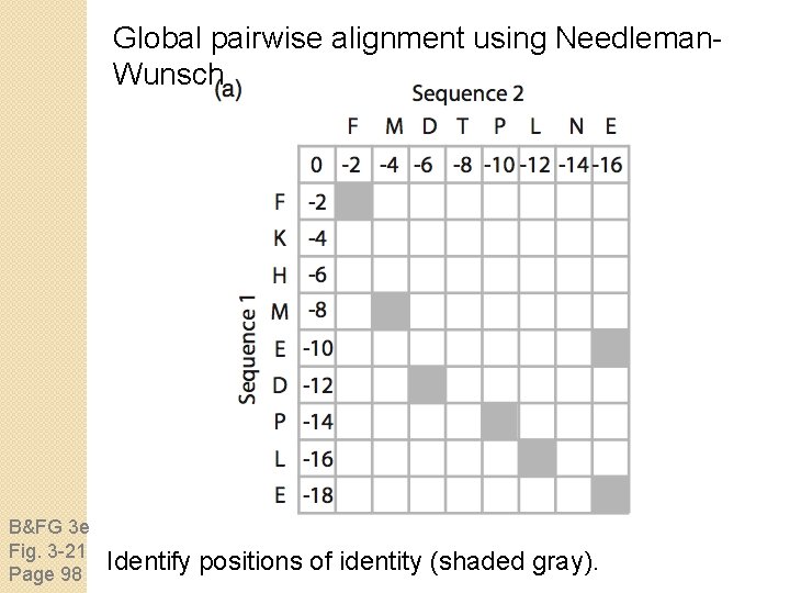
Global pairwise alignment using Needleman. Wunsch B&FG 3 e Fig. 3 -21 Page 98 Identify positions of identity (shaded gray).

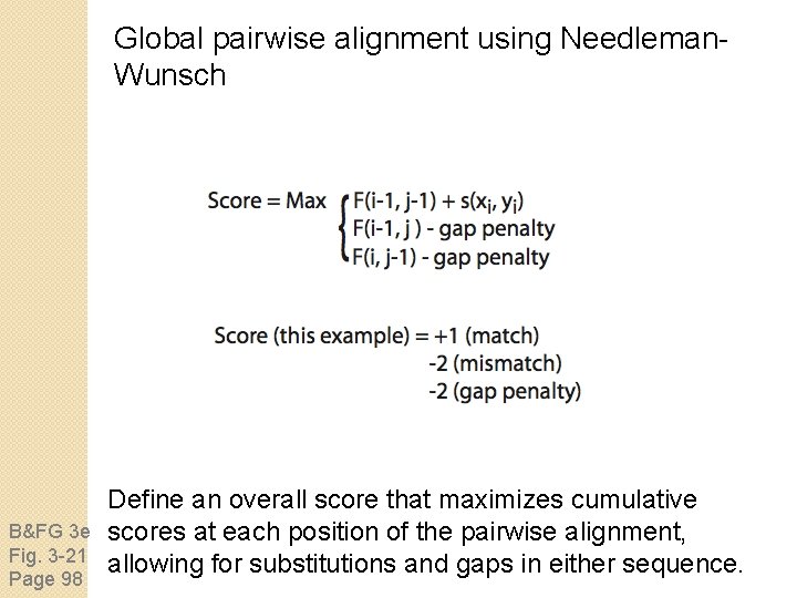
Global pairwise alignment using Needleman. Wunsch B&FG 3 e Fig. 3 -21 Page 98 Define an overall score that maximizes cumulative scores at each position of the pairwise alignment, allowing for substitutions and gaps in either sequence.

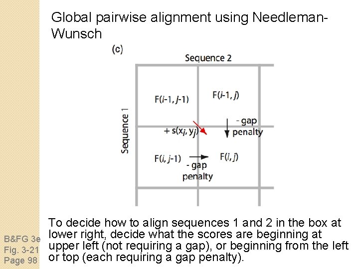
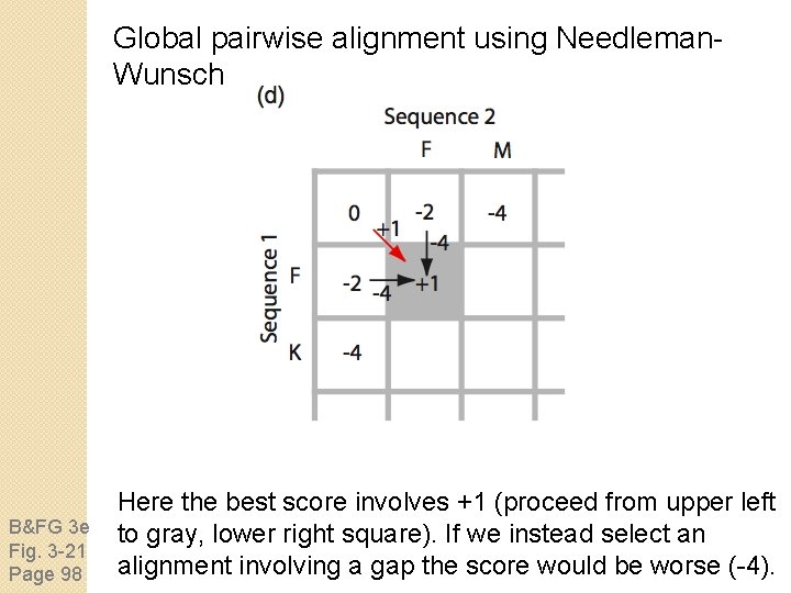
Global pairwise alignment using Needleman. Wunsch B&FG 3 e Fig. 3 -21 Page 98 To decide how to align sequences 1 and 2 in the box at lower right, decide what the scores are beginning at upper left (not requiring a gap), or beginning from the left or top (each requiring a gap penalty).

Global pairwise alignment using Needleman. Wunsch B&FG 3 e Fig. 3 -21 Page 98 Here the best score involves +1 (proceed from upper left to gray, lower right square). If we instead select an alignment involving a gap the score would be worse (-4).

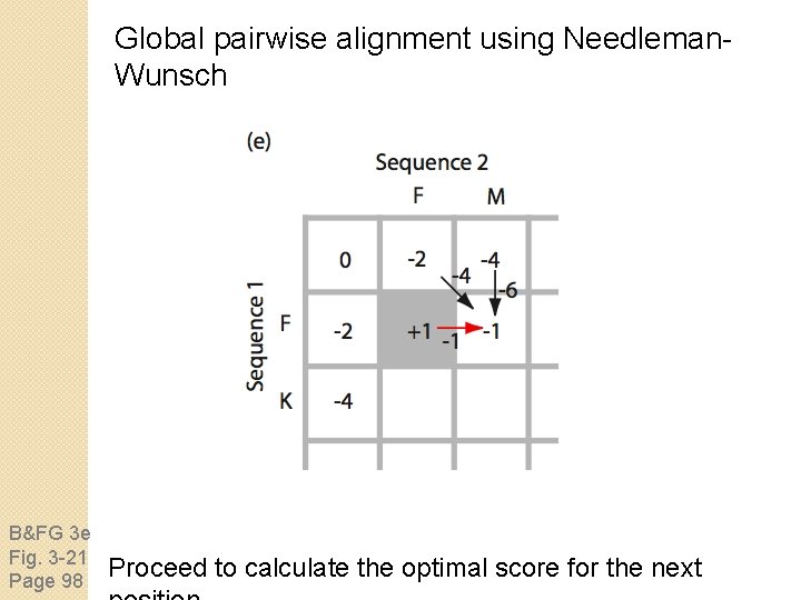
Global pairwise alignment using Needleman. Wunsch B&FG 3 e Fig. 3 -21 Page 98 Proceed to calculate the optimal score for the next

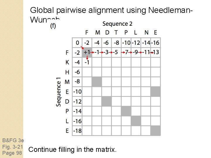
Global pairwise alignment using Needleman. Wunsch B&FG 3 e Fig. 3 -21 Page 98 Continue filling in the matrix.

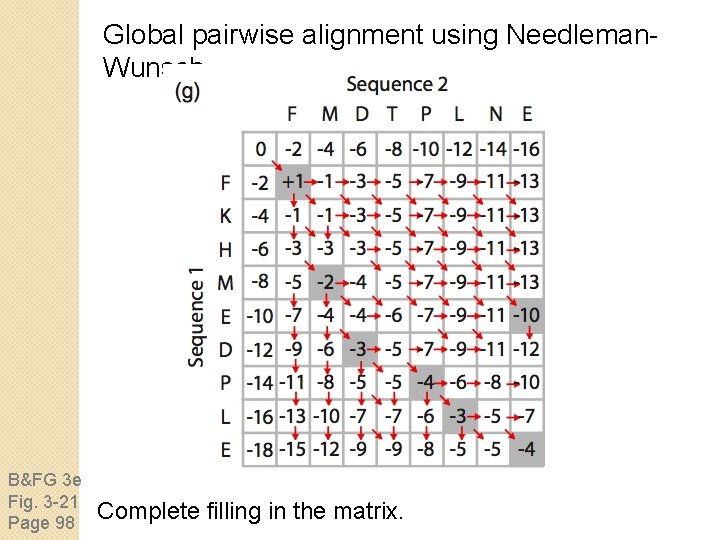
Global pairwise alignment using Needleman. Wunsch B&FG 3 e Fig. 3 -21 Page 98 Complete filling in the matrix.

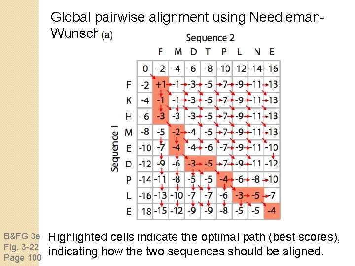
Global pairwise alignment using Needleman. Wunsch B&FG 3 e Fig. 3 -22 Page 100 Highlighted cells indicate the optimal path (best scores), indicating how the two sequences should be aligned.

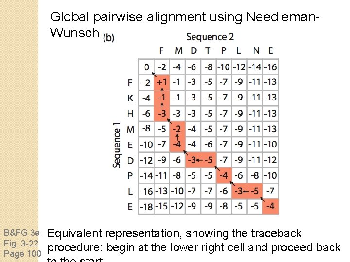
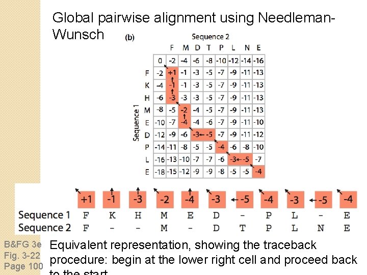
Global pairwise alignment using Needleman. Wunsch B&FG 3 e Fig. 3 -22 Page 100 Equivalent representation, showing the traceback procedure: begin at the lower right cell and proceed back

Global pairwise alignment using Needleman. Wunsch B&FG 3 e Fig. 3 -22 Page 100 Equivalent representation, showing the traceback procedure: begin at the lower right cell and proceed back

Needleman-Wunsch: dynamic programming N-W is guaranteed to find optimal alignments, although the algorithm does not search all possible alignments. It is an example of a dynamic programming algorithm: an optimal path (alignment) is identified by incrementally extending optimal subpaths. Thus, a series of decisions is made at each step of the alignment to find the pair of residues with the best score.

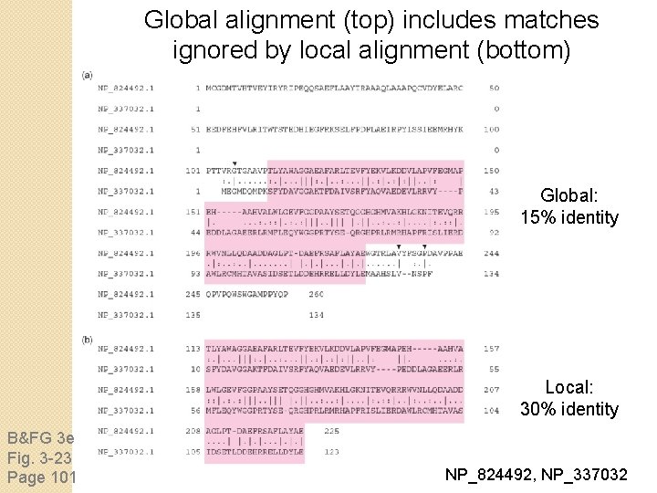
Global alignment versus local alignment Global alignment (Needleman-Wunsch) extends from one end of each sequence to the other. Local alignment finds optimally matching regions within two sequences (“subsequences”). Local alignment is almost always used for database searches such as BLAST. It is useful to find domains (or limited regions of homology) within sequences. Smith and Waterman (1981) solved the problem of performing optimal local sequence alignment. Other methods (BLAST, FASTA) are faster but less thorough.

Global alignment (top) includes matches ignored by local alignment (bottom) Global: 15% identity Local: 30% identity B&FG 3 e Fig. 3 -23 Page 101 NP_824492, NP_337032

Outline Introduction Protein alignment: often more informative than DNA alignment Definitions: homology, similarity, identity Gaps Pairwise alignment, homology, and evolution of life Scoring matrices Dayhoff model: 7 steps Pairwise alignment and limits of detection: the “twilight zone” Alignment algorithms: global and local Global sequence alignment: algorithm of Needleman and Wunsch Local sequence alignment: Smith and Waterman algorithm Rapid, heuristic versions of Smith–Waterman: FASTA and BLAST Basic Local Alignment Search Tool (BLAST) Pairwise alignment with dotplots The statistical significance of pairwise alignments Statistical significance of global alignments

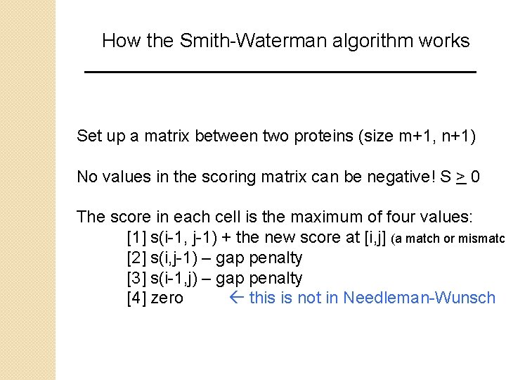
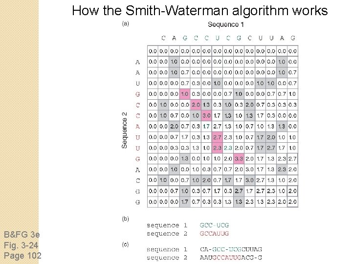
How the Smith-Waterman algorithm works Set up a matrix between two proteins (size m+1, n+1) No values in the scoring matrix can be negative! S > 0 The score in each cell is the maximum of four values: [1] s(i-1, j-1) + the new score at [i, j] (a match or mismatch [2] s(i, j-1) – gap penalty [3] s(i-1, j) – gap penalty [4] zero this is not in Needleman-Wunsch

How the Smith-Waterman algorithm works B&FG 3 e Fig. 3 -24 Page 102

Where to use the Smith-Waterman algorithm [1] Galaxy offers “needle” and “water” EMBOSS programs. [2] EBI offers needle and water. http: //www. ebi. ac. uk/Tools/psa/ [3] Try using SSEARCH to perform a rigorous Smith. Waterman local alignment: http: //fasta. bioch. virginia. edu/ [4] Next-generation sequence aligners incorporate Smith-Waterman in some specialized steps.

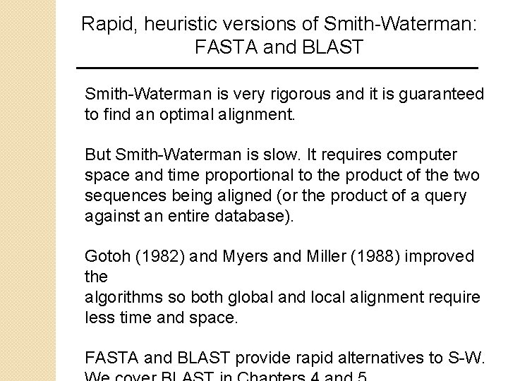
Rapid, heuristic versions of Smith-Waterman: FASTA and BLAST Smith-Waterman is very rigorous and it is guaranteed to find an optimal alignment. But Smith-Waterman is slow. It requires computer space and time proportional to the product of the two sequences being aligned (or the product of a query against an entire database). Gotoh (1982) and Myers and Miller (1988) improved the algorithms so both global and local alignment require less time and space. FASTA and BLAST provide rapid alternatives to S-W.

Outline Introduction Protein alignment: often more informative than DNA alignment Definitions: homology, similarity, identity Gaps Pairwise alignment, homology, and evolution of life Scoring matrices Dayhoff model: 7 steps Pairwise alignment and limits of detection: the “twilight zone” Alignment algorithms: global and local Global sequence alignment: algorithm of Needleman and Wunsch Local sequence alignment: Smith and Waterman algorithm Rapid, heuristic versions of Smith–Waterman: FASTA and BLAST Basic Local Alignment Search Tool (BLAST) Pairwise alignment with dotplots The statistical significance of pairwise alignments Statistical significance of global alignments

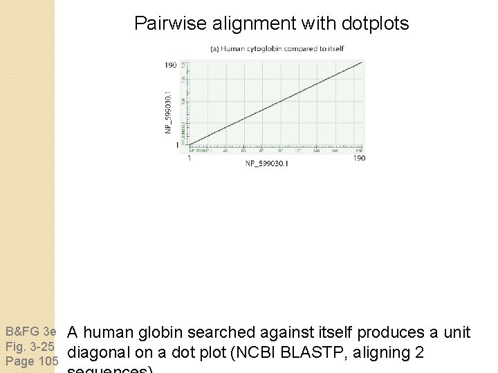
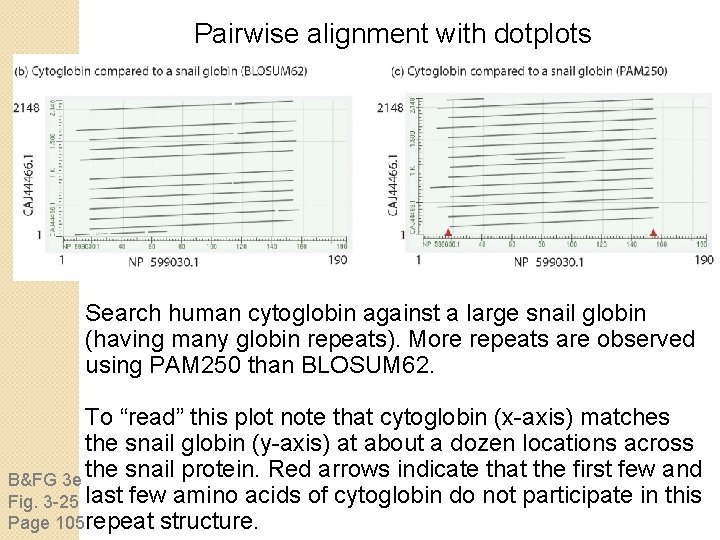
Pairwise alignment with dotplots B&FG 3 e Fig. 3 -25 Page 105 A human globin searched against itself produces a unit diagonal on a dot plot (NCBI BLASTP, aligning 2

Pairwise alignment with dotplots Search human cytoglobin against a large snail globin (having many globin repeats). More repeats are observed using PAM 250 than BLOSUM 62. To “read” this plot note that cytoglobin (x-axis) matches the snail globin (y-axis) at about a dozen locations across the snail protein. Red arrows indicate that the first few and B&FG 3 e Fig. 3 -25 last few amino acids of cytoglobin do not participate in this Page 105 repeat structure.

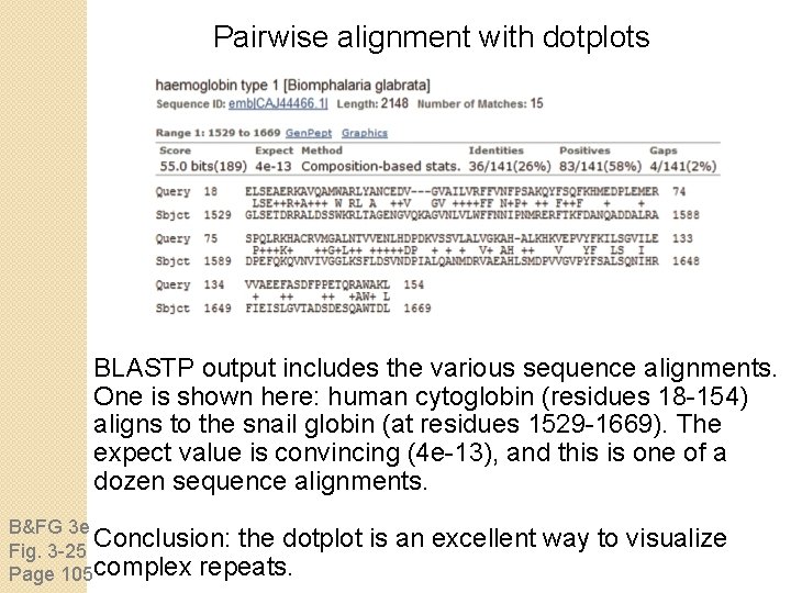
Pairwise alignment with dotplots BLASTP output includes the various sequence alignments. One is shown here: human cytoglobin (residues 18 -154) aligns to the snail globin (at residues 1529 -1669). The expect value is convincing (4 e-13), and this is one of a dozen sequence alignments. B&FG 3 e Conclusion: the dotplot Fig. 3 -25 Page 105 complex repeats. is an excellent way to visualize

Outline Introduction Protein alignment: often more informative than DNA alignment Definitions: homology, similarity, identity Gaps Pairwise alignment, homology, and evolution of life Scoring matrices Dayhoff model: 7 steps Pairwise alignment and limits of detection: the “twilight zone” Alignment algorithms: global and local Global sequence alignment: algorithm of Needleman and Wunsch Local sequence alignment: Smith and Waterman algorithm Rapid, heuristic versions of Smith–Waterman: FASTA and BLAST Basic Local Alignment Search Tool (BLAST) Pairwise alignment with dotplots The statistical significance of pairwise alignments Statistical significance of global alignments

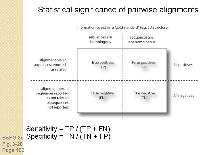
Statistical significance of pairwise alignments B&FG 3 e Fig. 3 -26 Page 106 Sensitivity = TP / (TP + FN) Specificity = TN / (TN + FP)

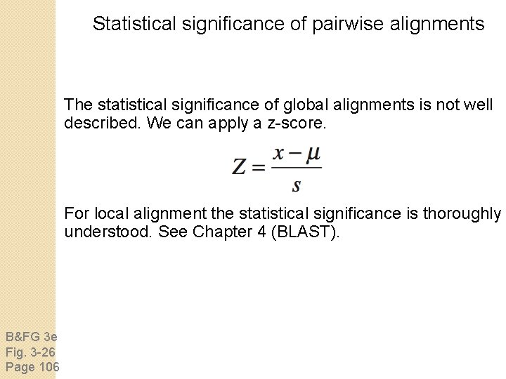
Statistical significance of pairwise alignments The statistical significance of global alignments is not well described. We can apply a z-score. For local alignment the statistical significance is thoroughly understood. See Chapter 4 (BLAST). B&FG 3 e Fig. 3 -26 Page 106

Outline Introduction Protein alignment: often more informative than DNA alignment Definitions: homology, similarity, identity Gaps Pairwise alignment, homology, and evolution of life Scoring matrices Dayhoff model: 7 steps Pairwise alignment and limits of detection: the “twilight zone” Alignment algorithms: global and local Global sequence alignment: algorithm of Needleman and Wunsch Local sequence alignment: Smith and Waterman algorithm Rapid, heuristic versions of Smith–Waterman: FASTA and BLAST Basic Local Alignment Search Tool (BLAST) Pairwise alignment with dotplots The statistical significance of pairwise alignments Statistical significance of global alignments

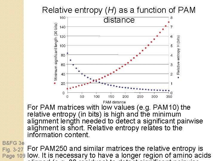
Relative entropy (H) as a function of PAM distance For PAM matrices with low values (e. g. PAM 10) the relative entropy (in bits) is high and the minimum alignment length needed to detect a significant pairwise alighment is short. Relative entropy relates to the information content. B&FG 3 e Fig. 3 -27 Page 109 For PAM 250 and similar matrices the relative entropy is low. It is necessary to have a longer region of amino acids

Perspective Pairwise alignment is a fundamental problem in bioinformatics. We discussed concepts of homology, and global versus local alignment (e. g. Needleman. Wunsch versus Smith-Waterman algorithms).

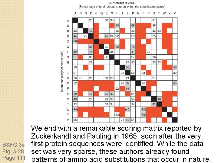
B&FG 3 e Fig. 3 -28 Page 111 We end with a remarkable scoring matrix reported by Zuckerkandl and Pauling in 1965, soon after the very first protein sequences were identified. While the data set was very sparse, these authors already found patterns of amino acid substitutions that occur in nature.