Advances and Limitations of Maximum Likelihood Phylogenetics Olivier

Advances and Limitations of Maximum Likelihood Phylogenetics Olivier Gascuel LIRMM-CNRS, Montpellier, France

Stéphane Guindon Wim Hordijk Quang Le Si Nicolas Lartillot Maria Anisimova Jean-François Dufayard

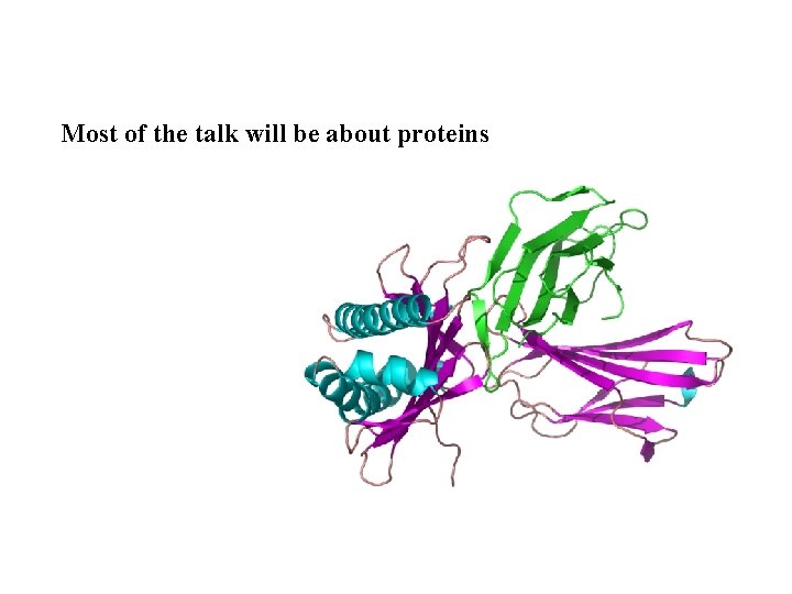
Most of the talk will be about proteins

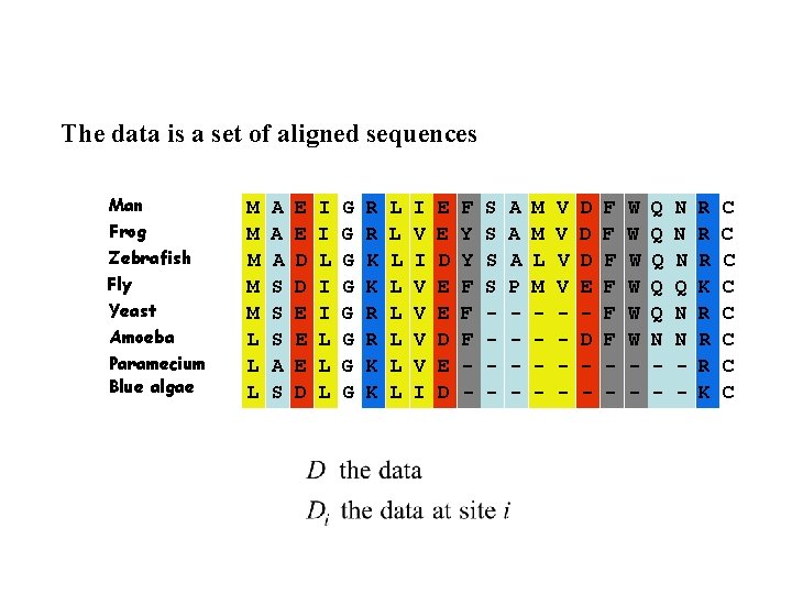
The data is a set of aligned sequences Man Frog Zebrafish Fly Yeast Amoeba Paramecium Blue algae M M M L L L A A A S S S A S E E D D E E E D I I L L L G G G G R R K K L L L L I V V V V I E E D E D F Y Y F F F - S S - A A A P - M M L M - V V - D D D E D - F F F - W W W - Q Q Q N - N N N Q N N - R R R K C C C C

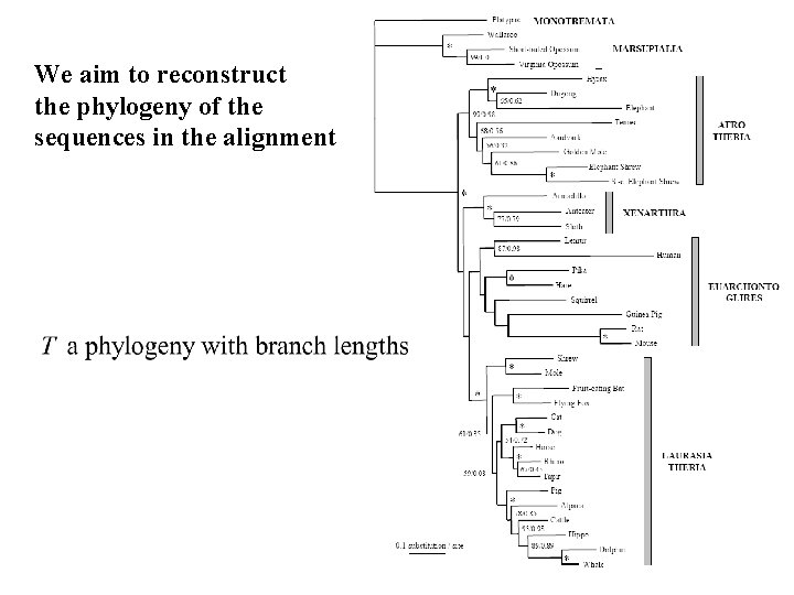
We aim to reconstruct the phylogeny of the sequences in the alignment

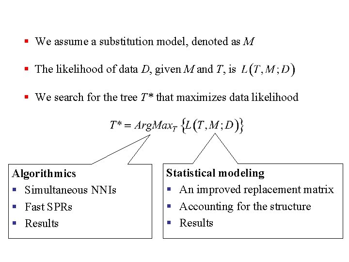
§ We assume a substitution model, denoted as M § The likelihood of data D, given M and T, is § We search for the tree T* that maximizes data likelihood Algorithmics § Simultaneous NNIs § Fast SPRs § Results Statistical modeling § An improved replacement matrix § Accounting for the structure § Results

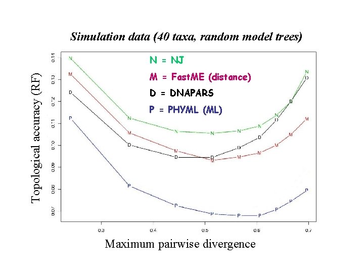
Simulation data (40 taxa, random model trees) Topological accuracy (RF) N = NJ M = Fast. ME (distance) D = DNAPARS P = PHYML (ML) Maximum pairwise divergence

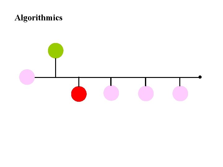
Algorithmics

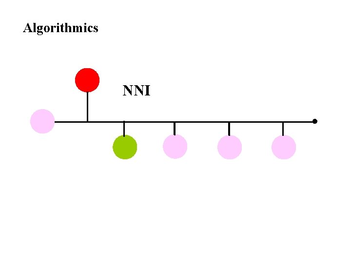
Algorithmics NNI

Algorithmics

Algorithmics

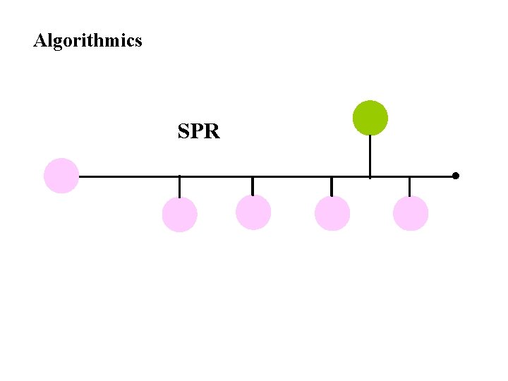
Algorithmics SPR

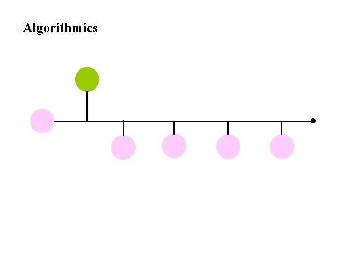
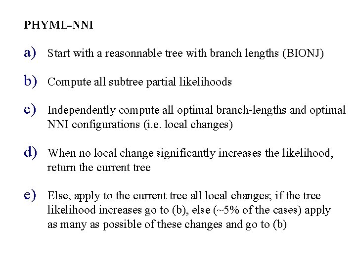
PHYML-NNI a) Start with a reasonnable tree with branch lengths (BIONJ) b) Compute all subtree partial likelihoods c) Independently compute all optimal branch-lengths and optimal NNI configurations (i. e. local changes) d) When no local change significantly increases the likelihood, return the current tree e) Else, apply to the current tree all local changes; if the tree likelihood increases go to (b), else (~5% of the cases) apply as many as possible of these changes and go to (b)

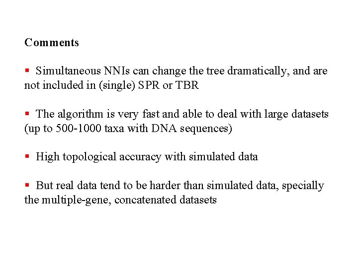
Comments § Simultaneous NNIs can change the tree dramatically, and are not included in (single) SPR or TBR § The algorithm is very fast and able to deal with large datasets (up to 500 -1000 taxa with DNA sequences) § High topological accuracy with simulated data § But real data tend to be harder than simulated data, specially the multiple-gene, concatenated datasets

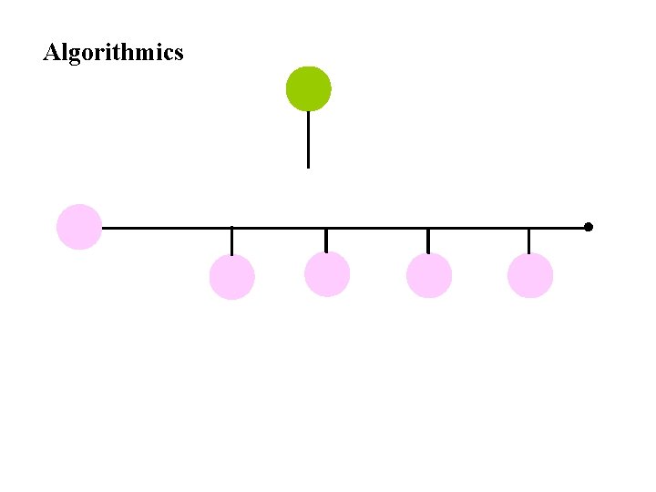
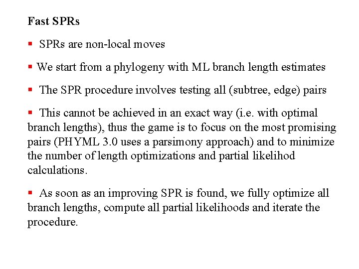
Fast SPRs § SPRs are non-local moves § We start from a phylogeny with ML branch length estimates § The SPR procedure involves testing all (subtree, edge) pairs § This cannot be achieved in an exact way (i. e. with optimal branch lengths), thus the game is to focus on the most promising pairs (PHYML 3. 0 uses a parsimony approach) and to minimize the number of length optimizations and partial likelihod calculations. § As soon as an improving SPR is found, we fully optimize all branch lengths, compute all partial likelihoods and iterate the procedure.

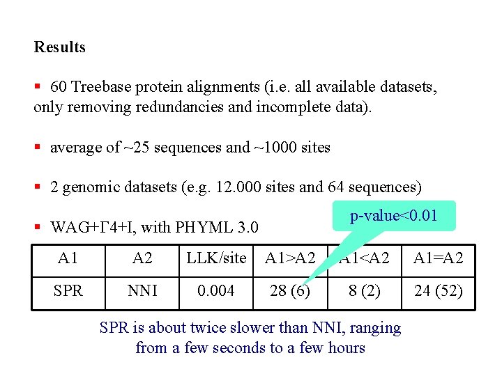
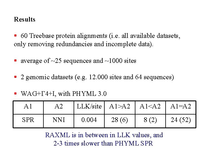
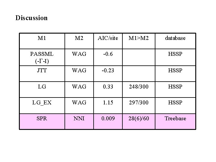
Results § 60 Treebase protein alignments (i. e. all available datasets, only removing redundancies and incomplete data). § average of ~25 sequences and ~1000 sites § 2 genomic datasets (e. g. 12. 000 sites and 64 sequences) p-value<0. 01 § WAG+G 4+I, with PHYML 3. 0 A 1 A 2 LLK/site A 1>A 2 A 1<A 2 A 1=A 2 SPR NNI 0. 004 28 (6) 8 (2) 24 (52) SPR is about twice slower than NNI, ranging from a few seconds to a few hours

Results § 60 Treebase protein alignments (i. e. all available datasets, only removing redundancies and incomplete data). § average of ~25 sequences and ~1000 sites § 2 genomic datasets (e. g. 12. 000 sites and 64 sequences) § WAG+G 4+I, with PHYML 3. 0 A 1 A 2 LLK/site A 1>A 2 A 1<A 2 A 1=A 2 SPR NNI 0. 004 28 (6) 8 (2) 24 (52) RAXML is in between in LLK values, and 2 -3 times slower than PHYML SPR

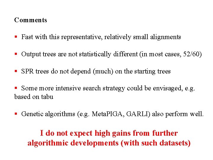
Comments § Fast with this representative, relatively small alignments § Output trees are not statistically different (in most cases, 52/60) § SPR trees do not depend (much) on the starting trees § Some more intensive search strategy could be envisaged, e. g. based on tabu § Genetic algorithms (e. g. Meta. PIGA, GARLI) also perform well. I do not expect high gains from further algorithmic developments (with such datasets)

Statistical modeling § An improved, general AA replacement matrix § Accounting for structure and exposition to solvent § Results

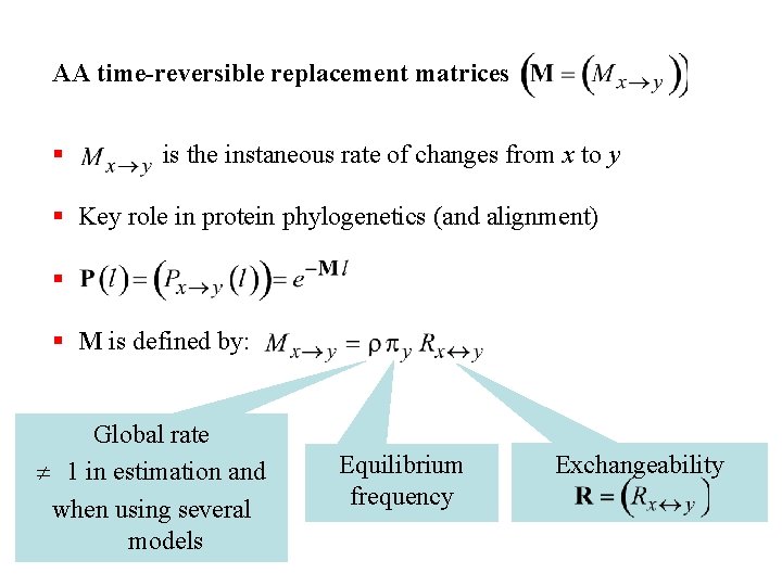
AA time-reversible replacement matrices § is the instaneous rate of changes from x to y § Key role in protein phylogenetics (and alignment) § § M is defined by: Global rate 1 in estimation and when using several models Equilibrium frequency Exchangeability

Estimating replacement matrices § Counting approach of Dayhoff et al. (1972), using pairwise alignments of closely related proteins (PAM, JTT, …). § Logarithmic (Gonnet et al 1992) and resolvent (Muller et al 2000) counting approaches to deal with pairs of remote proteins § A strong tendency is to estimate different matrices for different protein groups (mitochondrial, prokaryotic, viral, arthropoda …). § But general matrices (e. g. , JTT, WAG) are widely used, e. g. to build deep phylogenies or to analyze concatenated datasets.

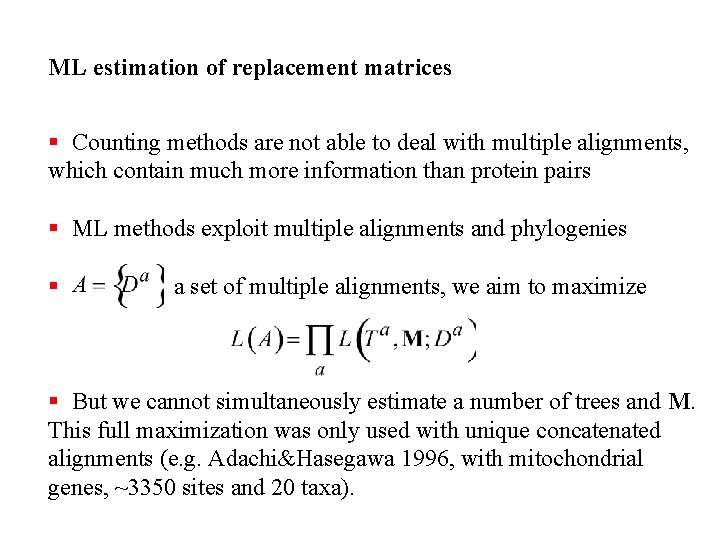
ML estimation of replacement matrices § Counting methods are not able to deal with multiple alignments, which contain much more information than protein pairs § ML methods exploit multiple alignments and phylogenies § a set of multiple alignments, we aim to maximize § But we cannot simultaneously estimate a number of trees and M. This full maximization was only used with unique concatenated alignments (e. g. Adachi&Hasegawa 1996, with mitochondrial genes, ~3350 sites and 20 taxa).

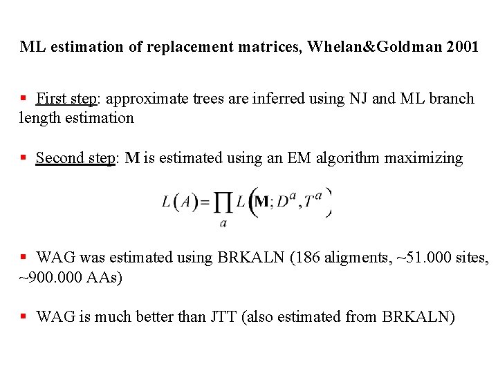
ML estimation of replacement matrices, Whelan&Goldman 2001 § First step: approximate trees are inferred using NJ and ML branch length estimation § Second step: M is estimated using an EM algorithm maximizing § WAG was estimated using BRKALN (186 aligments, ~51. 000 sites, ~900. 000 AAs) § WAG is much better than JTT (also estimated from BRKALN)

ML estimation of replacement matrices, Whelan&Goldman 2001 § Variability of rates across sites (RAS) was not incorporated in likelihood calculations. § It is now recognized that RAS is essential. Some sites are slow (invariant) due to strong evolutionary constraints, while others are very fast. § RAS is usually implemented with a discrete gamma distribution of rates and invariant sites (G 4+I), and used to infer most of trees. § Moreover, BRKALN is limited regarding current databases, and likely biased toward proteins being easy to cristallize, with well defined 3 D structure.

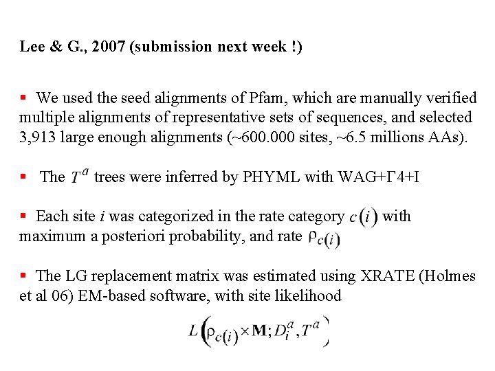
Lee & G. , 2007 (submission next week !) § We used the seed alignments of Pfam, which are manually verified multiple alignments of representative sets of sequences, and selected 3, 913 large enough alignments (~600. 000 sites, ~6. 5 millions AAs). § The trees were inferred by PHYML with WAG+G 4+I § Each site i was categorized in the rate category maximum a posteriori probability, and rate with § The LG replacement matrix was estimated using XRATE (Holmes et al 06) EM-based software, with site likelihood

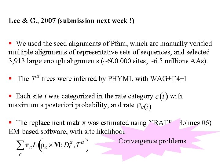
Lee & G. , 2007 (submission next week !) § We used the seed alignments of Pfam, which are manually verified multiple alignments of representative sets of sequences, and selected 3, 913 large enough alignments (~600. 000 sites, ~6. 5 millions AAs). § The trees were inferred by PHYML with WAG+G 4+I § Each site i was categorized in the rate category maximum a posteriori probability, and rate with § The replacement matrix was estimated using XRATE (Holmes 06) EM-based software, with site likelihood Convergence problems

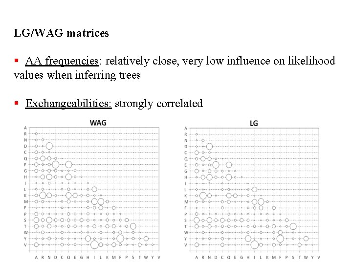
LG/WAG matrices § AA frequencies: relatively close, very low influence on likelihood values when inferring trees § Exchangeabilities: strongly correlated

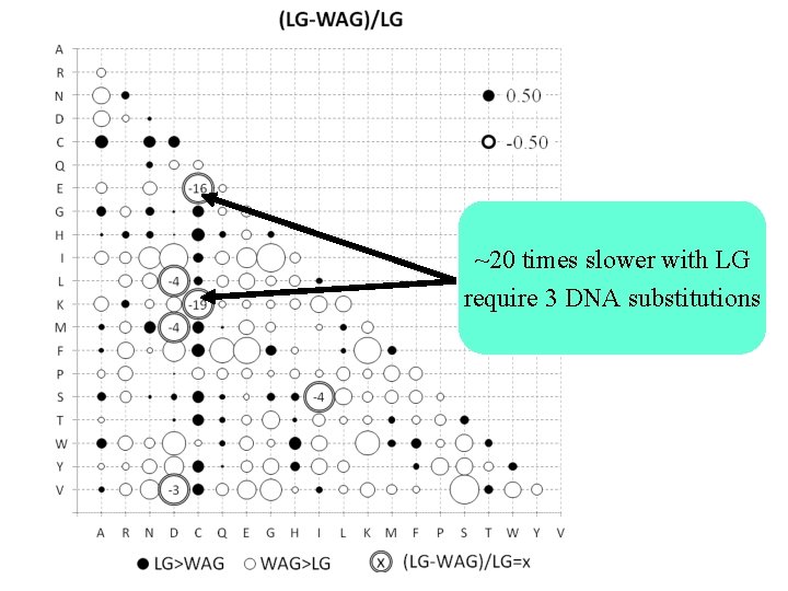
~20 times slower with LG require 3 DNA substitutions

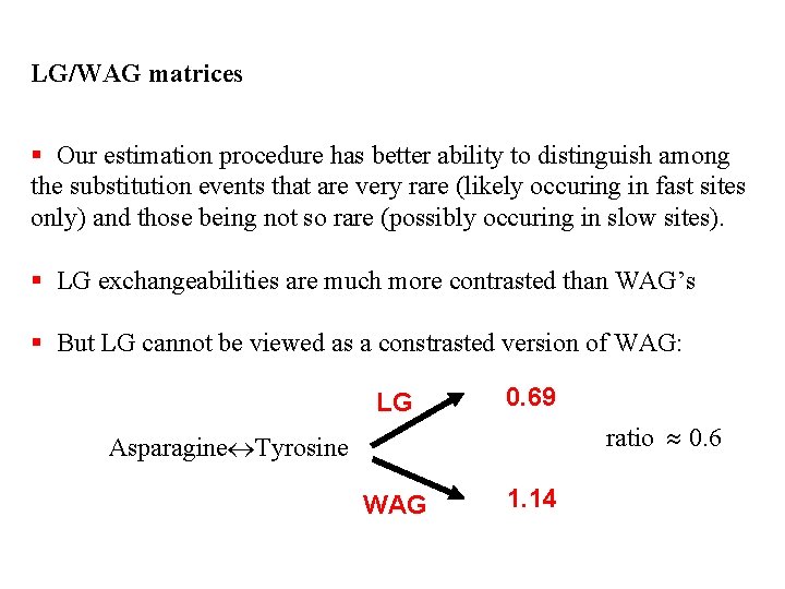
LG/WAG matrices § Our estimation procedure has better ability to distinguish among the substitution events that are very rare (likely occuring in fast sites only) and those being not so rare (possibly occuring in slow sites). § LG exchangeabilities are much more contrasted than WAG’s § But LG cannot be viewed as a constrasted version of WAG: LG 0. 69 ratio 0. 6 Asparagine Tyrosine WAG 1. 14

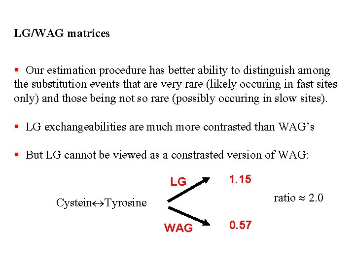
LG/WAG matrices § Our estimation procedure has better ability to distinguish among the substitution events that are very rare (likely occuring in fast sites only) and those being not so rare (possibly occuring in slow sites). § LG exchangeabilities are much more contrasted than WAG’s § But LG cannot be viewed as a constrasted version of WAG: LG 1. 15 ratio 2. 0 Cystein Tyrosine WAG 0. 57

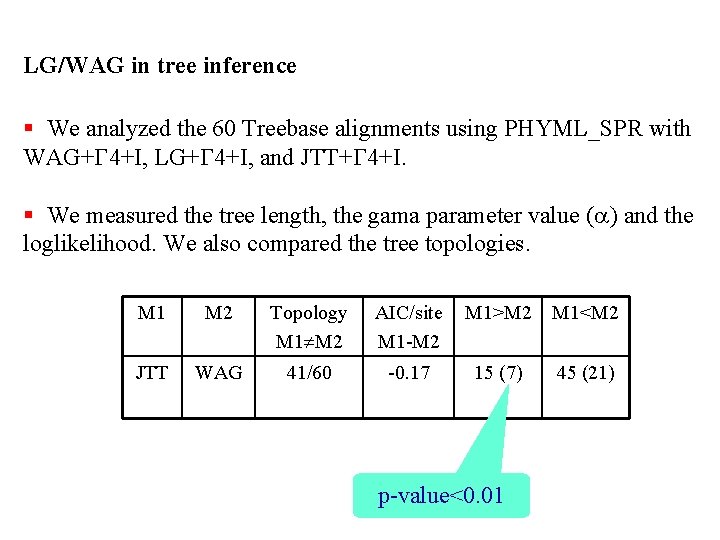
LG/WAG in tree inference § We analyzed the 60 Treebase alignments using PHYML_SPR with WAG+G 4+I, LG+G 4+I, and JTT+G 4+I. § We measured the tree length, the gama parameter value (a) and the loglikelihood. We also compared the tree topologies. M 1 M 2 Topology M 1 M 2 AIC/site M 1 -M 2 M 1>M 2 M 1<M 2 JTT WAG 41/60 -0. 17 15 (7) 45 (21) p-value<0. 01

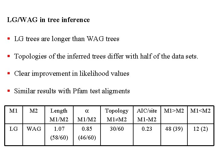
LG/WAG in tree inference § LG trees are longer than WAG trees § Topologies of the inferred trees differ with half of the data sets. § Clear improvement in likelihood values § Similar results with Pfam test aligments M 1 M 2 Length M 1/M 2 a M 1/M 2 Topology M 1 M 2 AIC/site M 1 -M 2 M 1>M 2 M 1<M 2 LG WAG 1. 07 (58/60) 0. 85 (46/60) 30/60 0. 23 48 (39) 12 (2)

Accounting for exposition and secondary structure § Substitutions clearly depend on secondary structure and exposition; e. g. , buried sites are and remain hydrophobic. § Overington et al. 1990; Lüthy et al. 1991; Topham et al. 1993; Wako and Blundell 1994; Goldman et al. 1996 (to infer both the structure and the phylogeny). § Not (or rarely) used today in phylogenetics, though the structure of dozens of thousands of proteins is now available. § We revisited the question thanks to (1) our improved ML-based estimation procedure, (2) the huge, current databases.

Learning and testing data § We extracted from HSSP ((homology-derived structures of proteins) 4, 889 non-redundant (sub)alignments. § 290, 000 sequences, 1, 250, 000 sites and 71 billions AAs. § Secondary structure (Helix, Sheet, Turn, Coil) and exposition (Exposed, Buried) are available for all the sites, but not fully reliable (80 -90% of conservation). § We randomly selected 500 alignments as a test set, leaving 4, 389 alignments to learn substitution matrices for various site categories ( E, B; H, S, T, C; E&H, E&S, E&T …).

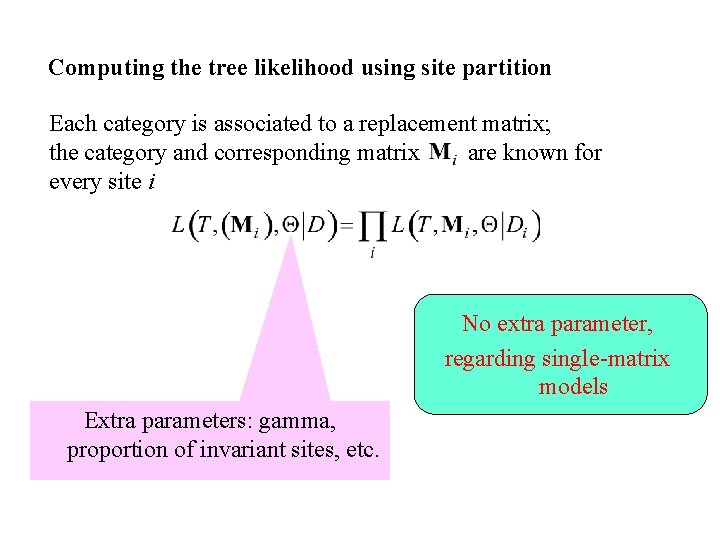
Computing the tree likelihood using site partition Each category is associated to a replacement matrix; the category and corresponding matrix are known for every site i No extra parameter, regarding single-matrix models Extra parameters: gamma, proportion of invariant sites, etc.

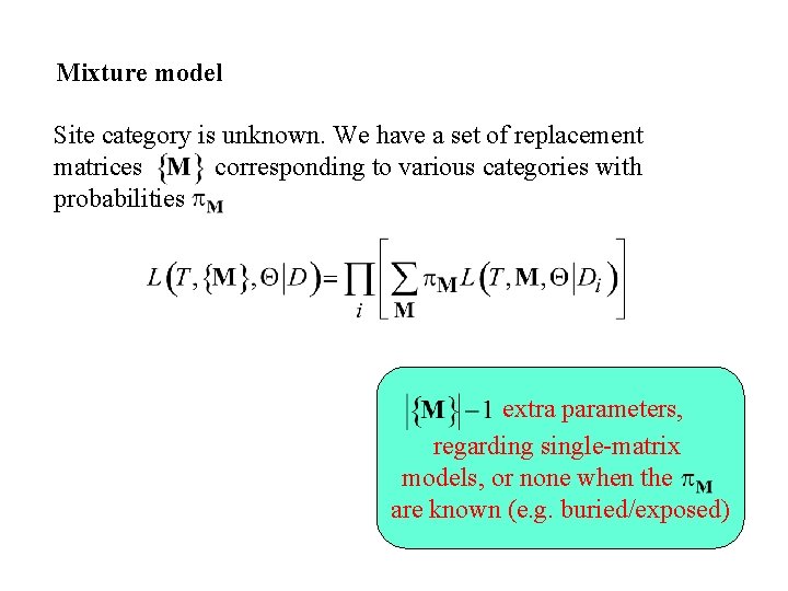
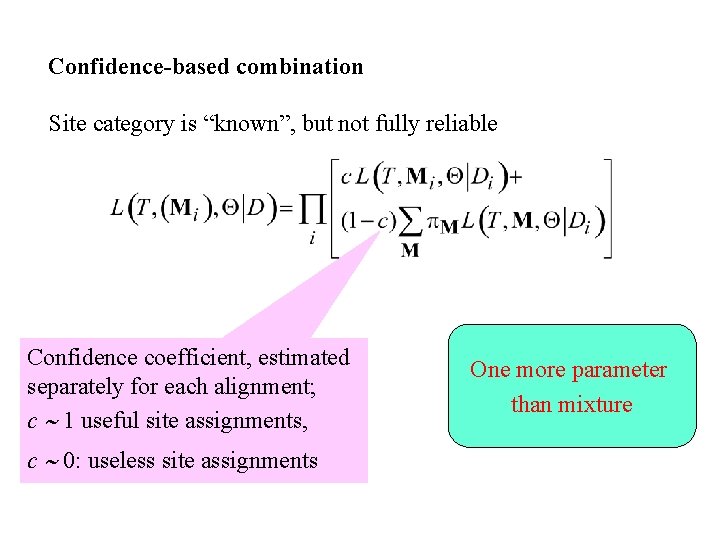
Mixture model Site category is unknown. We have a set of replacement matrices corresponding to various categories with probabilities extra parameters, regarding single-matrix models, or none when the are known (e. g. buried/exposed)

Confidence-based combination Site category is “known”, but not fully reliable Confidence coefficient, estimated separately for each alignment; c 1 useful site assignments, c 0: useless site assignments One more parameter than mixture

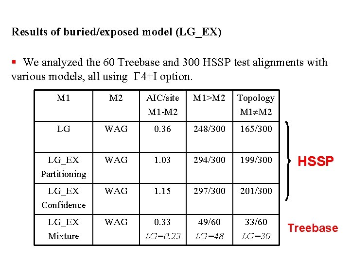
Results of buried/exposed model (LG_EX) § We analyzed the 60 Treebase and 300 HSSP test alignments with various models, all using G 4+I option. M 1 M 2 AIC/site M 1 -M 2 M 1>M 2 Topology M 1 M 2 LG WAG 0. 36 248/300 165/300 LG_EX Partitioning WAG 1. 03 294/300 199/300 LG_EX Confidence WAG 1. 15 297/300 201/300 LG_EX Mixture WAG 0. 33 LG=0. 23 49/60 LG=48 33/60 LG=30 HSSP Treebase

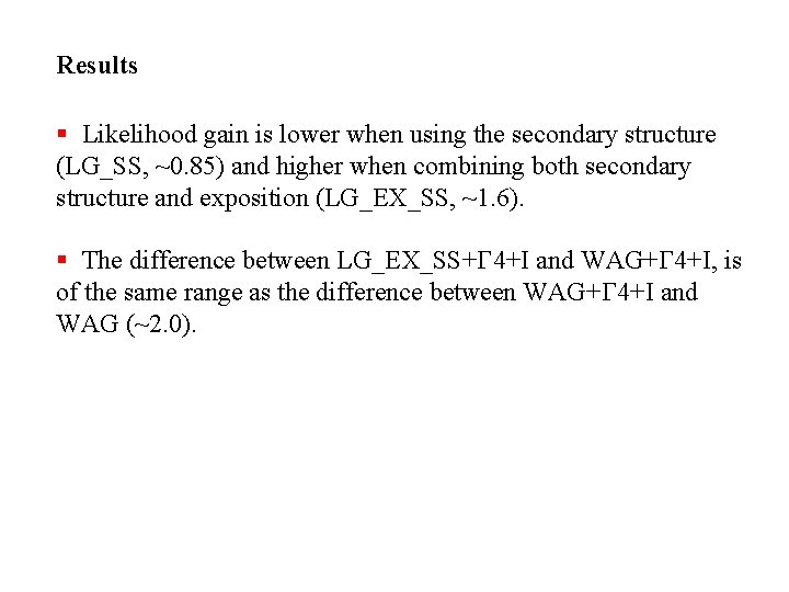
Results § Likelihood gain is lower when using the secondary structure (LG_SS, ~0. 85) and higher when combining both secondary structure and exposition (LG_EX_SS, ~1. 6). § The difference between LG_EX_SS+G 4+I and WAG+G 4+I, is of the same range as the difference between WAG+G 4+I and WAG (~2. 0).

Discussion We revisited questions and models which were proposed and explored by N. Goldman, Z. Yang, their collaborators, … others, using today § concepts, e. g. RAS MUST be accounted for in tree inference AND replacement matrix estimation, § tools (XRATE, PHYML), § and databases (Pfam, HSSP).

Discussion We revisited questions and models which were proposed and explored by N. Goldman, Z. Yang, their collaborators, … others, using today § concepts, e. g. RAS MUST be accounted for in tree inference AND replacement matrix estimation, § tools (XRATE, PHYML), § and databases (Pfam, HSSP), § and computers !

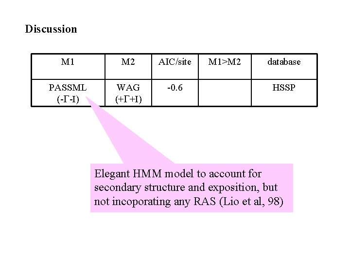
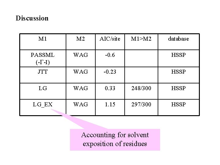
Discussion M 1 M 2 AIC/site PASSML (-G-I) WAG (+G+I) -0. 6 M 1>M 2 database HSSP Elegant HMM model to account for secondary structure and exposition, but not incoporating any RAS (Lio et al, 98)

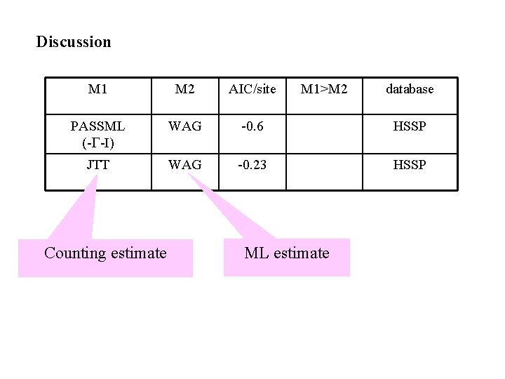
Discussion M 1 M 2 AIC/site PASSML (-G-I) WAG -0. 6 HSSP JTT WAG -0. 23 HSSP Counting estimate M 1>M 2 ML estimate database

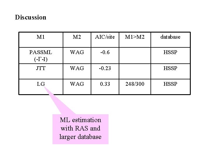
Discussion M 1 M 2 AIC/site PASSML (-G-I) WAG -0. 6 HSSP JTT WAG -0. 23 HSSP LG WAG 0. 33 ML estimation with RAS and larger database M 1>M 2 248/300 database HSSP

Discussion M 1 M 2 AIC/site M 1>M 2 PASSML (-G-I) WAG -0. 6 HSSP JTT WAG -0. 23 HSSP LG WAG 0. 33 248/300 HSSP LG_EX WAG 1. 15 297/300 HSSP Accounting for solvent exposition of residues database

Discussion M 1 M 2 AIC/site M 1>M 2 database PASSML (-G-I) WAG -0. 6 HSSP JTT WAG -0. 23 HSSP LG WAG 0. 33 248/300 HSSP LG_EX WAG 1. 15 297/300 HSSP SPR NNI 0. 009 28(6)/60 Treebase

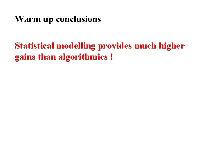
Warm up conclusions Statistical modelling provides much higher gains than algorithmics !

Warm up conclusions Statistical modelling provides much higher gains than algorithmics ! This should continue in the next years, as current models are still rejected for a number of alignments …….

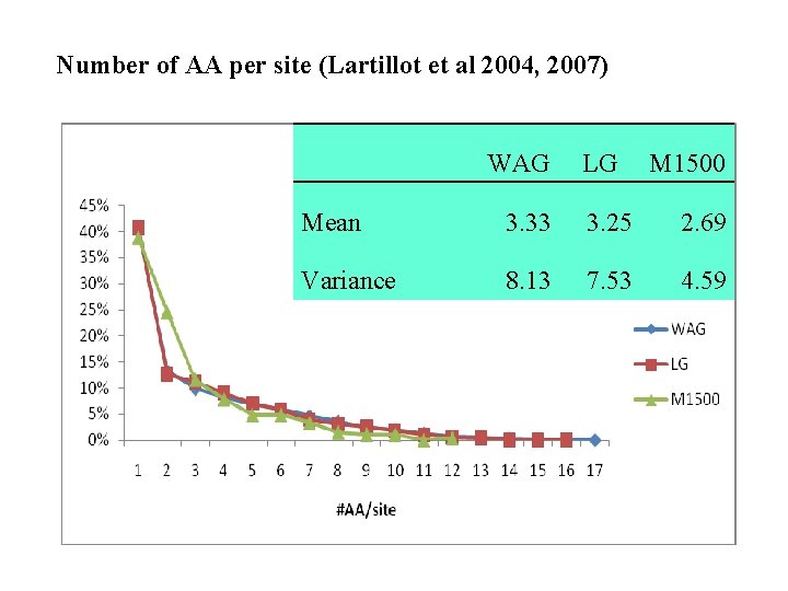
Number of AA per site (Lartillot et al 2004, 2007) WAG LG M 1500 Mean 3. 33 3. 25 2. 69 Variance 8. 13 7. 53 4. 59

Warm up conclusions Statistical modelling provides much higher gains than algorithmics ! This should continue in the next years, as current models are still rejected for a number of alignments …. .

Thank you all, the organizers and the Isaac Newton Institute

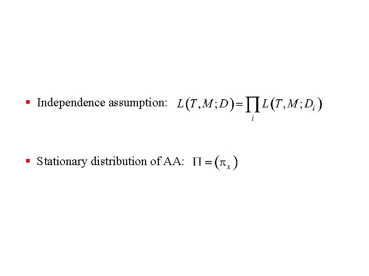
§ Independence assumption: § Stationary distribution of AA:

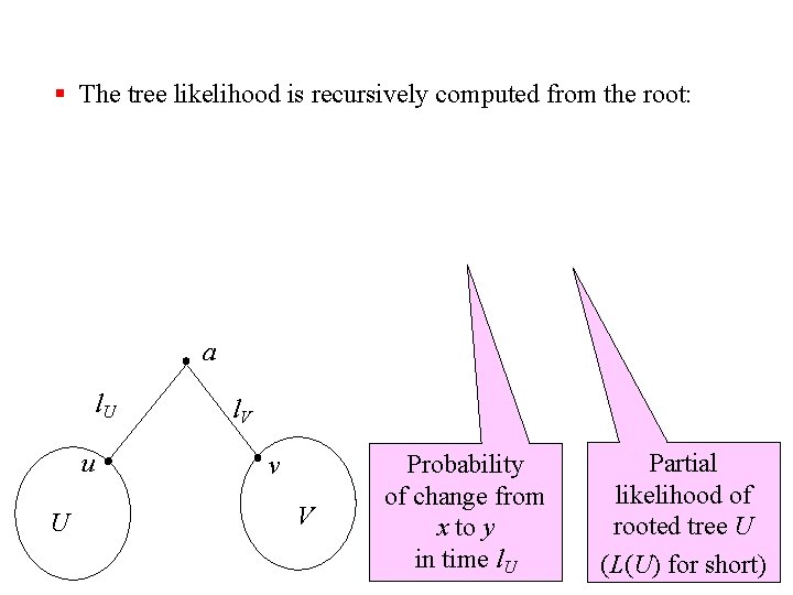
§ The tree likelihood is recursively computed from the root: a l. U u U l. V v V Probability of change from x to y in time l. U Partial likelihood of rooted tree U (L(U) for short)

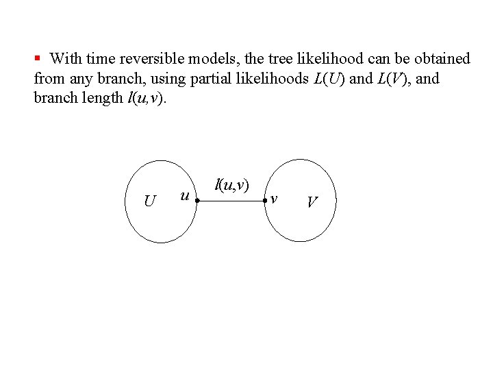
§ With time reversible models, the tree likelihood can be obtained from any branch, using partial likelihoods L(U) and L(V), and branch length l(u, v). U u l(u, v) v V

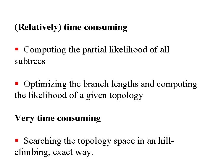
(Relatively) time consuming § Computing the partial likelihood of all subtrees § Optimizing the branch lengths and computing the likelihood of a given topology Very time consuming § Searching the topology space in an hillclimbing, exact way.

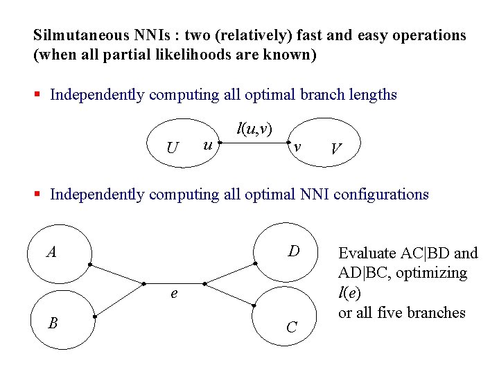
Silmutaneous NNIs : two (relatively) fast and easy operations (when all partial likelihoods are known) § Independently computing all optimal branch lengths U u l(u, v) v V § Independently computing all optimal NNI configurations D A e B C Evaluate AC|BD and AD|BC, optimizing l(e) or all five branches

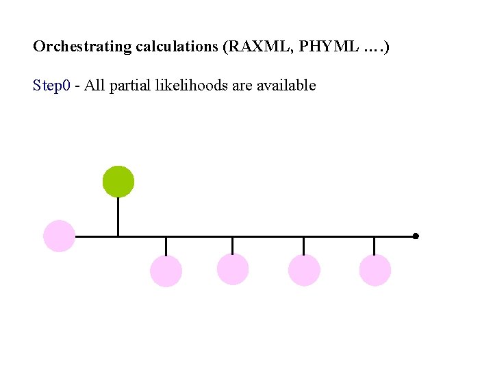
Orchestrating calculations (RAXML, PHYML …. ) Step 0 - All partial likelihoods are available

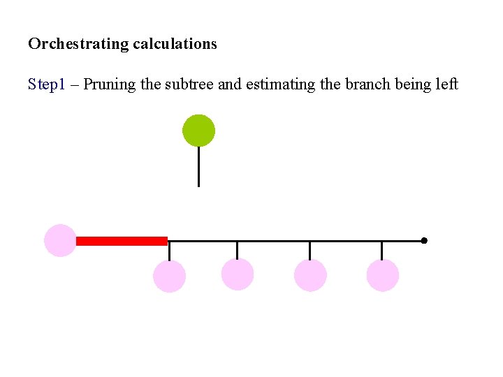
Orchestrating calculations Step 1 – Pruning the subtree and estimating the branch being left

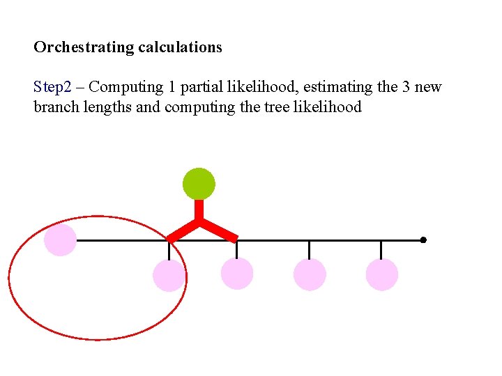
Orchestrating calculations Step 2 – Computing 1 partial likelihood, estimating the 3 new branch lengths and computing the tree likelihood

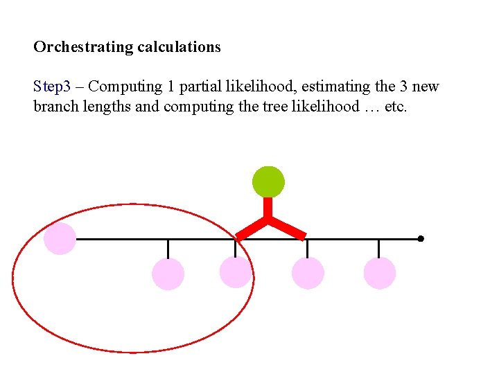
Orchestrating calculations Step 3 – Computing 1 partial likelihood, estimating the 3 new branch lengths and computing the tree likelihood … etc.

Progressive filtering strategy (PHYML) § All possible SPRs are first filtered by a fast distance-based (or parsimony) algorithm; typically, we retain for every subtree the 20% most promising edges for regraphting. § Previous scheme is run several times with increasingly sophisticated branch-length estimations; when an improving SPR is found, it is returned and the procedure restart from the beginning; else, results are used to rank and filter remaining SPRs. § This strategy allows considerable gain in computing time, without loss on the resulting tree.