Ad hoc and Sensor Networks Unit 3 Network

Ad hoc and Sensor Networks Unit 3: Network architecture

Outline • • • Network scenarios Optimization goals Design principles Service interface Gateway concepts

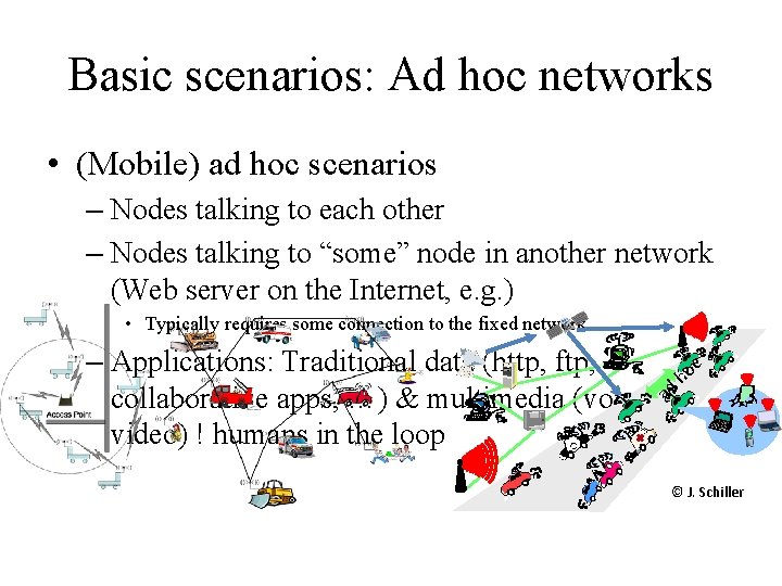
Basic scenarios: Ad hoc networks • (Mobile) ad hoc scenarios – Nodes talking to each other – Nodes talking to “some” node in another network (Web server on the Internet, e. g. ) • Typically requires some connection to the fixed network c – Applications: Traditional data (http, ftp, ho collaborative apps, …) & multimedia (voice, ad video) ! humans in the loop © J. Schiller

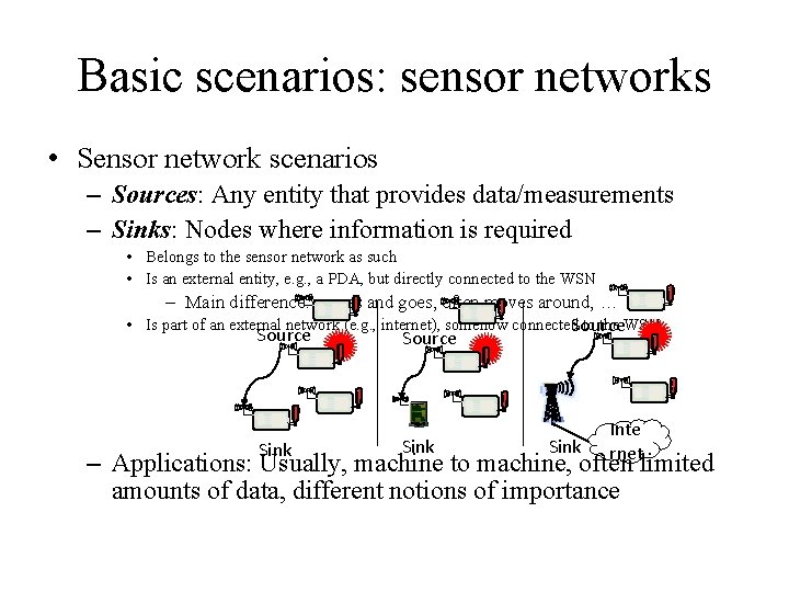
Basic scenarios: sensor networks • Sensor network scenarios – Sources: Any entity that provides data/measurements – Sinks: Nodes where information is required • Belongs to the sensor network as such • Is an external entity, e. g. , a PDA, but directly connected to the WSN – Main difference: comes and goes, often moves around, … • Is part of an external network (e. g. , internet), somehow connected. Source to the WSN Source Sink Inte rnet – Applications: Usually, machine to machine, often limited amounts of data, different notions of importance

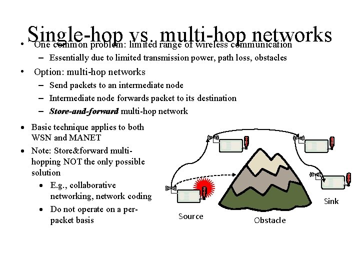
Single-hop vs. multi-hop networks • One common problem: limited range of wireless communication – Essentially due to limited transmission power, path loss, obstacles • Option: multi-hop networks – Send packets to an intermediate node – Intermediate node forwards packet to its destination – Store-and-forward multi-hop network · Basic technique applies to both WSN and MANET · Note: Store&forward multihopping NOT the only possible solution · E. g. , collaborative networking, network coding · Do not operate on a perpacket basis Sink Source Obstacle

Energy efficiency of multi-hopping? • Obvious idea: Multi-hopping is more energy-efficient than direct communication – Because of path loss > 2, energy for distance d is reduced from cd to 2 c(d/2) • c some constant • However: This is usually wrong, or at least very oversimplified – Need to take constant offsets for powering transmitter, receiver into account – Details see exercise, chapter 2 ! Multi-hopping for energy savings needs careful choice

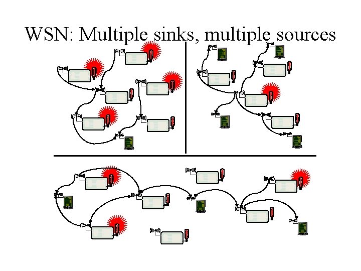
WSN: Multiple sinks, multiple sources

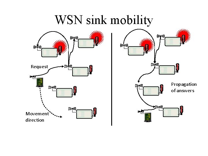
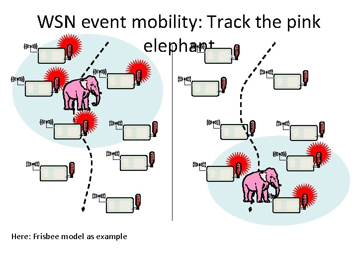
Different sources of mobility • Node mobility – A node participating as source/sink (or destination) or a relay node might move around – Deliberately, self-propelled or by external force; targeted or at random – Happens in both WSN and MANET • Sink mobility – In WSN, a sink that is not part of the WSN might move – Mobile requester • Event mobility – In WSN, event that is to be observed moves around (or extends, shrinks) – Different WSN nodes become “responsible” for surveillance of such an event

WSN sink mobility Request Propagation of answers Movement direction

WSN event mobility: Track the pink elephant Here: Frisbee model as example

Outline • • • Network scenarios Optimization goals Design principles Service interface Gateway concepts

Optimization goal: Quality of Service • In MANET: Usual Qo. S interpretation – Throughput/delay/jitter – High perceived Qo. S for multimedia applications • In WSN, more complicated – – Event detection/reporting probability Event classification error, detection delay Probability of missing a periodic report Approximation accuracy (e. g, when WSN constructs a temperature map) – Tracking accuracy (e. g. , difference between true and conjectured position of the pink elephant) • Related goal: robustness – Network should withstand failure of some nodes

Optimization goal: Energy efficiency • Umbrella term! • Energy per correctly received bit – Counting all the overheads, in intermediate nodes, etc. • Energy per reported (unique) event – After all, information is important, not payload bits! – Typical for WSN • Delay/energy tradeoffs • Network lifetime – – – Time to first node failure Network half-life (how long until 50% of the nodes died? ) Time to partition Time to loss of coverage Time to failure of first event notification

Optimization goal: Energy efficiency • Much of the discussion has already shown that energy is a precious resource in wireless sensor networks and that energy efficiency should therefore make an evident optimization goal. • There should be reasonable understanding of the term energy efficiency. • The term “energy efficiency” is, in fact, rather an umbrella term for many different aspects of a system, which should be carefully distinguished to form actual, measurable figures of merit. • The most commonly considered aspects are: 1) Energy per correctly received bit: How much energy, counting all sources of energy consumption at all possible intermediate hops, is spent on average to transport one bit of information (payload) from the source to the destination?

Optimization goal: Energy efficiency 2) Energy per reported (unique) event: Similarly, what is the average energy spent to report one event? Since the same event is sometimes reported from various sources, it is usual to normalize this metric to only the unique events. 3) Delay/energy trade-offs: Some applications have a notion of “urgent” events, which can justify an increased energy investment for a speedy reporting of such events. Here, the trade-off between delay and energy overhead is interesting. 4) Network lifetime: The time for which the network is operational or, put another way, the time during which it is able to fulfill its tasks. It is not quite clear, however, when this time ends. Possible definitions are:

Optimization goal: Energy efficiency a) Time to first node death: When does the first node in the network run out of energy or fail and stop operating? b) Network half-life: When have 50% of the nodes run out of energy and stopped operating? Any other fixed percentile is applicable as well. c) Time to partition: When does the first partition of the network in two (or more) disconnected parts occur? This can be as early as the death of the first node (if that was in a pivotal position) or occur very late if the network topology is robust. d) Time to loss of coverage: Usually, with redundant network deployment and sensors that can observe a region instead of just the very spot where the node is located, each point in the deployment region is observed by multiple sensor nodes. A possible figure of merit is thus the time when for the first time any spot in the deployment region is no longer covered by any node’s observations.

Optimization goal: Energy efficiency • If k redundant observations are necessary (for tracking applications, for example), the corresponding definition of loss of coverage would be the first time any spot in the deployment region is no longer covered by at least k different sensor nodes. e) Time to failure of first event notification: A network partition can be seen as irrelevant if the unreachable part of the network does not want to report any events in the first place. • Hence, a possibly more application-specific interpretation of partition is the inability to deliver an event. • This can be due to an event not being noticed because the responsible sensor is dead or because a partition between source and sink has occurred. • All these metrics can of course only be evaluated under a clear set of assumptions about the energy consumption characteristics of a given node, about the actual “load” that the network has to deal with (e. g. when and where do events happen), and also about the behavior of the radio channel.

Optimization goal: Scalability • Network should be operational regardless of number of nodes – At high efficiency • Typical node numbers difficult to guess – MANETs: 10 s to 100 s – WSNs: 10 s to 1000 s, maybe more • Requiring to scale to large node numbers has serious consequences for network architecture – Might not result in the most efficient solutions for small networks! – Architectures and protocols should implement appropriate scalability support rather than trying to be as scalable as possible.

Optimization goal: Robustness • Related to Qo. S and somewhat also to scalability requirements, wireless sensor networks should also exhibit an appropriate robustness. • They should not fail just because a limited number of nodes run out of energy, or because their environment changes and affects existing radio links between two nodes. • If possible, these failures have to be compensated for, for example, by finding other routes. • A precise evaluation of robustness is difficult in practice and depends mostly on failure models for both nodes and communication links.

Outline • • • Network scenarios Optimization goals Design principles Service interface Gateway concepts

Design Principles for WSN • Appropriate Qo. S support, energy efficiency, and scalability are important design and optimization goals for wireless sensor networks. • But these goals themselves do not provide many hints on how to structure a network such that they are achieved. • A few basic principles have emerged, which can be useful when designing networking protocols.

Distributed organization • Participants in a MANET/WSN should cooperate in organizing the network – E. g. , with respect to medium access, routing, … – Centralistic approach as alternative usually not feasible – hinders scalability, robustness • Potential shortcomings – Not clear whether distributed or centralistic organization achieves better energy efficiency (when taking all overheads into account) • Option: “limited centralized” solution – Elect nodes for local coordination/control – Perhaps rotate this function over time

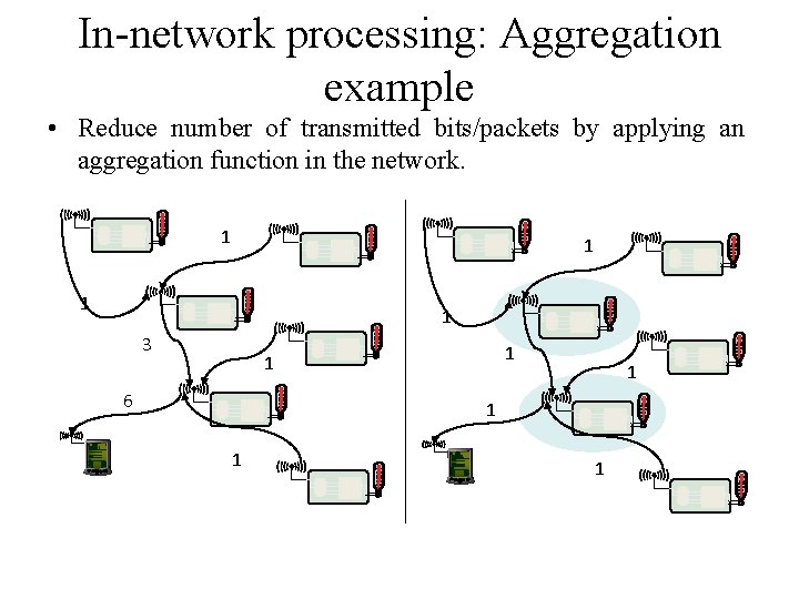
In-network processing • MANETs are supposed to deliver bits from one end to the other • WSNs, on the other end, are expected to provide information, not necessarily original bits – Gives addition options – E. g. , manipulate or process the data in the network • Main example: aggregation – Apply composable aggregation functions to a convergecast tree in a network – Typical functions: minimum, maximum, average, sum, … – Not amenable functions: median

In-network processing: Aggregation example • Reduce number of transmitted bits/packets by applying an aggregation function in the network. 1 1 3 1 1 6 1 1

Distributed source coding and distributed compression • Aggregation condenses and sacrifices information about the measured values in order not to have to transmit all bits of data from all sources to the sink. • Is it possible to reduce the number of transmitted bits but still obtain the full information about all sensor readings at the sink? • It is related to the coding and compression problems known from conventional networks, where a lot of effort is invested to encode, for example, a video sequence, to reduce the required bandwidth. • How can the fact that information is provided by multiple sensors be exploited to help in coding? • Some implicit, joint information between two sensors is required. • Recall here that these sensors are embedded in a physical environment – it is quite likely that the readings of adjacent sensors are going to be quite similar; they are correlated.

Distributed source coding and distributed compression • Such correlation can indeed be exploited such that not simply the sum of the data must be transmitted but that overhead can be saved here. • Exploit temporal and spatial correlation – Observed signals might vary only slowly in time ! no need to transmit all data at full rate all the time – Signals of neighboring nodes are often quite similar ! only try to transmit differences (details a bit complicated, see later)

In-network processing: signal processing • The in-networking processing approaches discussed so far have not really used the ability for processing in the sensor nodes, or have only used this for trivial operations like averaging or finding the maximum. • When complex computations on a certain amount of data is to be done, it can still be more energy efficient to compute these functions on the sensor nodes despite their limited processing power, • if in return the amount of data that has to be communicated can be reduced. • An example for this concept is the distributed computation of a Fast Fourier Transform (FFT).

In-network processing: signal processing • Depending on where the input data is located, there are different algorithms available to compute an FFT in a distributed fashion, with different trade-offs between local computation complexity and the need for communication. • A FFT Algorithm computes the Discrete F T of a sequence or its inverse. Fourier Analysis converts a signal from its original domain (time or space) to a representation in the frequency domain and vice versa. • Such distributed computations are mostly applicable to signal processing type algorithms; typical examples are beamforming and target tracking applications.

In-network processing: Mobile code/Agent-based networking • With the possibility of executing programs in the network, other programming paradigms or computational models are feasible. • One such model is the idea of mobile code or agent-based networking. • The idea is to have a small, compact representation of program code that is small enough to be sent from node to node. • This code is then executed locally, for example, collecting measurements, and then decides where to be sent next. • This idea has been used in various environments; a classic • example is that of a software agent that is sent out to collect the best possible travel itinerary by hopping from one travel agent’s computer to another and eventually returning to the user who has posted this inquiry. • In wireless sensor networks, mobile agents and related concepts have been considered in various contexts, mostly with respect to routing of queries and for data fusion, virtual machines for WSN etc.

Adaptive fidelity • Adapt the effort with which data is exchanged to the currently required accuracy/fidelity • Example event detection – When there is no event, only very rarely send short “all is well” messages – When event occurs, increase rate of message exchanges • Example temperature – When temperature is in acceptable range, only send temperature values at low resolution – When temperature becomes high, increase resolution and thus message length

Data centric networking • In typical networks (including ad hoc networks), network transactions are addressed to the identities of specific nodes – A “node-centric” or “address-centric” networking paradigm • In a redundantly deployed sensor networks, specific source of an event, alarm, etc. might not be important – Redundancy: e. g. , several nodes can observe the same area • Thus: focus networking transactions on the data directly instead of their senders and transmitters ! data-centric networking – Principal design change

Implementation options for data-centric networking • Overlay networks & distributed hash tables (DHT) – Hash table: content-addressable memory – Retrieve data from an unknown source, like in peer-to-peer networking – with efficient implementation – Some disparities remain • Static key in DHT, dynamic changes in WSN • DHTs typically ignore issues like hop count or distance between nodes when performing a lookup operation • Publish/subscribe – – Different interaction paradigm Nodes can publish data, can subscribe to any particular kind of data Once data of a certain type has been published, it is delivered to all subscribes Subscription and publication are decoupled in time; subscriber and published are agnostic of each other (decoupled in identity) • Databases

Further design principles • Exploit location information – Required anyways for many applications; can considerably increase performance • Exploit activity patterns • Exploit heterogeneity – By construction: nodes of different types in the network – By evolution: some nodes had to perform more tasks and have less energy left; some nodes received more solar energy than others; … • Cross-layer optimization of protocol stacks for WSN – Goes against grain of standard networking; but promises big performance gains – Also applicable to other networks like ad hoc; usually at least worthwhile to consider for most wireless networks

Outline • • • Network scenarios Optimization goals Design principles Service interface Gateway concepts

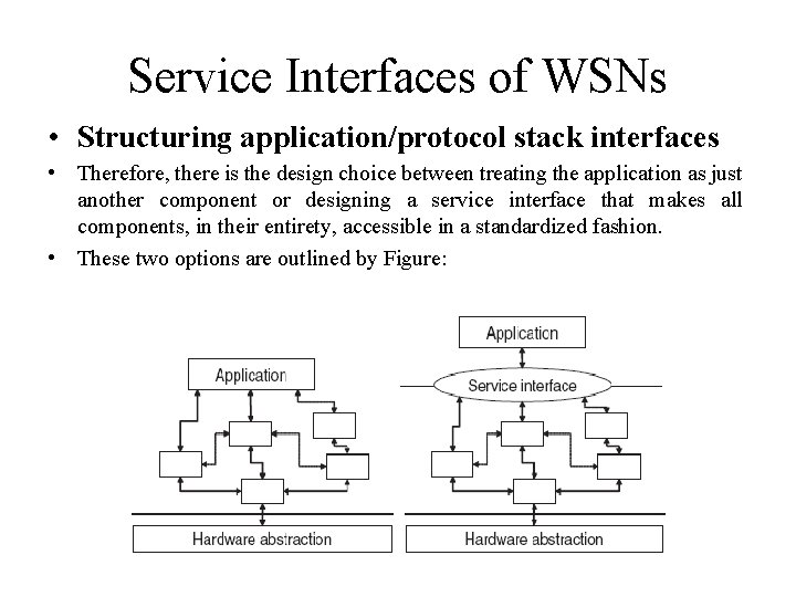
Service Interfaces of WSNs • Structuring application/protocol stack interfaces • a component-based operating system and protocol stack already enables one possibility to treat an application: • It is just another component that can directly interact with other components using whatever interface specification exists between them (e. g. The command/event structure of Tiny. OS). • The application could even consist of several components, integrated at various places into the protocol stack.

Service Interfaces of WSNs • • Structuring application/protocol stack interfaces This approach has several advantages: It is streamlined with the overall protocol structure, makes it easy to introduce application-specific code into the WSN at various levels, • and does not require the definition of an abstract, specific service interface. • Moreover, such a tight integration allows the application programmer a very fine-grained control over which protocols (which components) are chosen for a specific task; • for example, it is possible to select out of different routing protocols the one best suited for a given application by accessing this component’s services.

Service Interfaces of WSNs • Structuring application/protocol stack interfaces • But this generality and flexibility is also the potential downside of this approach. • The allowing of the application programmer to mess with protocol stacks and operating system internals should not be undertaken carelessly. • In traditional networks such as the Internet, the application programmer can access the services of the network via a commonly accepted interface: sockets. • This interface makes clear provisions on how to handle connections, how to send and receive packets, and how to inquire about state information of the network. • This clarity is owing to the evident tasks that this interface serves – the exchange of packets with one (sometimes, several) communication peers.

Service Interfaces of WSNs • Structuring application/protocol stack interfaces • Therefore, there is the design choice between treating the application as just another component or designing a service interface that makes all components, in their entirety, accessible in a standardized fashion. • These two options are outlined by Figure:

Service Interfaces of WSNs • Structuring application/protocol stack interfaces • A service interface would allow to raise the level of abstraction with which an application can interact with the WSN – instead of having to specify which value to read from which particular sensor, • it might be desirable to provide an application with the possibility to express sensing tasks in terms that are close to the semantics of the application. • In this sense, such a service interface can hide considerable complexity and is actually conceivable as a “middleware” in its own right. • The question is therefore on the one hand the price of standardization with respect to the potential loss of performance and on the other hand, the complexity of the service interface. • To better understand this trade-off, a clearer understanding of expressibility requirements of such an interface is necessary.

Service Interfaces of WSNs • Expressibility requirements for WSN service interfaces • • • Support for simple request/response interactions: retrieving a measured value from some sensor or setting a parameter in some node. This is a synchronous interaction pattern in the sense that the result (or possibly the acknowledgment) is expected immediately. In addition, the responses can be required to be provided periodically, supporting periodic measurement-type applications. Support for asynchronous event notifications: a requesting node can require the network to inform it if a given condition becomes true, for example, if a certain event has happened. This is an asynchronous pattern in the sense that there is no a priori relationship between the time the request is made and the time the information is provided. For both types of interactions, the addressees should be definable in several ways. The simplest option is an explicit enumeration of the single or multiple communication peers to whom a (synchronous or asynchronous) request is made – this corresponds to the peer address in a socket communication.

Service Interfaces of WSNs • • • More interesting is the question of how to express data centricity. One option, closely related to the publish/subscribe approach is the implicit definition of peers by some form of a membership function of an abstract group of nodes. Possible examples for such membership functions include: • Location – all nodes that are in a given region of space belong to a group. • Observed value – all nodes that have observed values matching a given predicate belong to a group. An example would be to require the measured temperature to be larger than 20◦C. In-networking processing functionality has to be accessible. For an operation that accesses an entire group of nodes, especially when reading values from this group (either synchronously or asynchronously), it should be possible to specify what kind of in-network processing should be applied to it. In particular, processing that modifies the nature of the result (i. e. , data fusion) must be explicitly allowed by the requesting application.

Service Interfaces of WSNs • • Related to the specification of aggregation functions is the specification of the required accuracy of a result. This can take on the form of specifying bounds on the number of group members that should contribute to a result, or the level of compression that should be applied. Hand in hand with required accuracy goes the acceptable energy expenditure to produce a given piece of information. Timeliness requirements about the delivery of data is a similar aspect. For example, it may be possible to provide a result quickly but at higher energy costs (e. g. by forcing nodes to wake up earlier than they would wake up anyway) or slowly but at reduced energy costs (e. g. By piggy-backing information on other data packets that have to exchanged anyway). The need to access location, timing, or network status information via the service interface. To support the seamless connection of various nodes or entire networks as well as the simple access to services in an “unknown” network, there is a need for an explicit description of the set of available capabilities of the node/the network.

Service Interfaces of WSNs • • Security requirements as well as properties have to be somehow expressed. While not a direct part of an actual service interface, additional management functionality, for example, for updating components, can be convenient to be present in the interface as well.

Outline • • • Network scenarios Optimization goals Design principles Service interface Gateway concepts

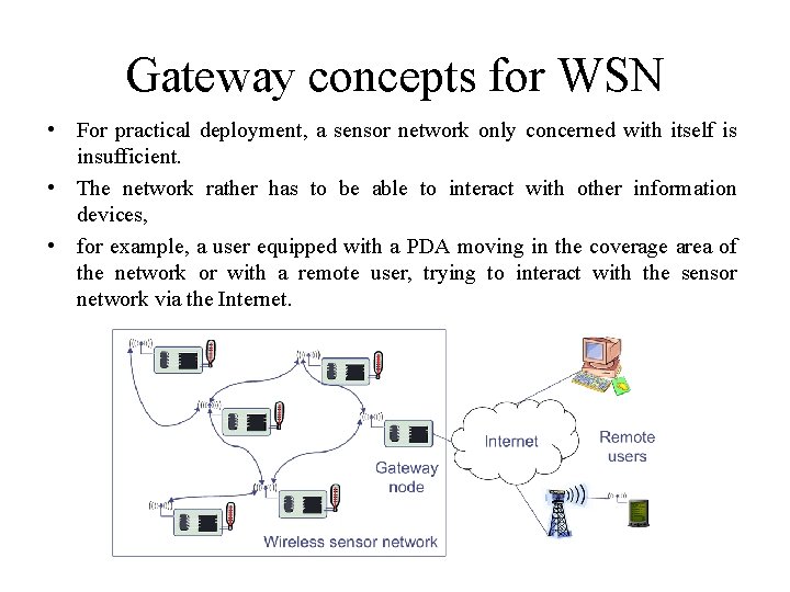
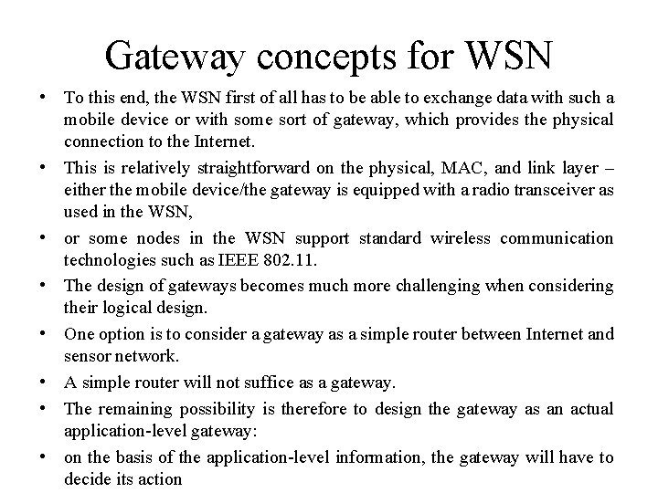
Gateway concepts for WSN • For practical deployment, a sensor network only concerned with itself is insufficient. • The network rather has to be able to interact with other information devices, • for example, a user equipped with a PDA moving in the coverage area of the network or with a remote user, trying to interact with the sensor network via the Internet.

Gateway concepts for WSN • To this end, the WSN first of all has to be able to exchange data with such a mobile device or with some sort of gateway, which provides the physical connection to the Internet. • This is relatively straightforward on the physical, MAC, and link layer – either the mobile device/the gateway is equipped with a radio transceiver as used in the WSN, • or some nodes in the WSN support standard wireless communication technologies such as IEEE 802. 11. • The design of gateways becomes much more challenging when considering their logical design. • One option is to consider a gateway as a simple router between Internet and sensor network. • A simple router will not suffice as a gateway. • The remaining possibility is therefore to design the gateway as an actual application-level gateway: • on the basis of the application-level information, the gateway will have to decide its action

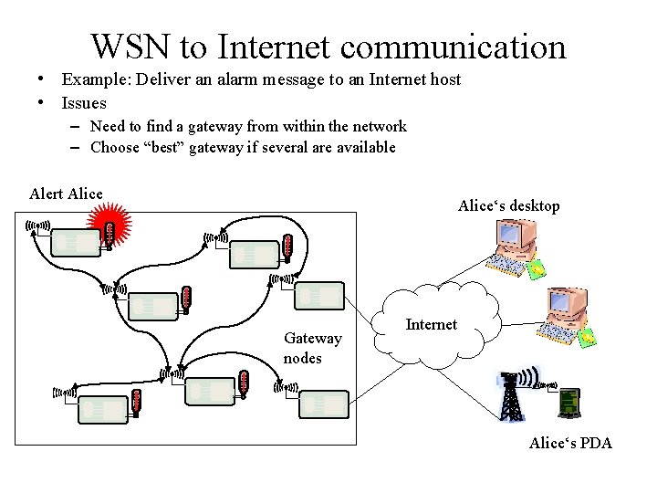
WSN to Internet communication • Example: Deliver an alarm message to an Internet host • Issues – Need to find a gateway from within the network – Choose “best” gateway if several are available Alert Alice‘s desktop Gateway nodes Internet Alice‘s PDA

WSN to Internet communication • In particular, if not all Internet hosts are reachable via each gateway or at least if some gateway should be preferred for a given destination host? • How to handle several gateways, each capable of IP networking, and the communication among them? • One option is to build an IP overlay network on top of the sensor network. • How does a sensor node know to which Internet host to address such a message? • Or even worse, how to map a semantic notion (“Alert Alice”) to a concrete IP address? • Even if the sensor node does not need to be able to process the IP protocol, it has to include sufficient information (IP address and port number, for example) in its own packets; the gateway then has to extract this information and translate it into IP packets. • An ensuing question is which source address to use here – the gateway in a sense has to perform tasks similar to that of a Network Address Translation (NAT) device.

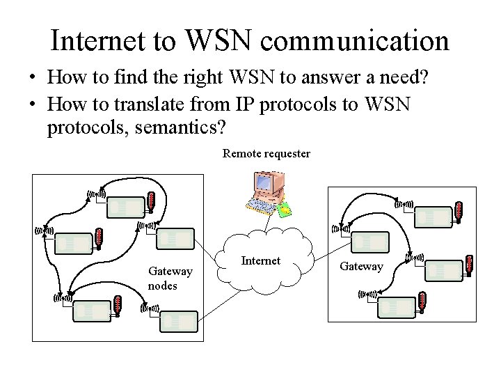
Internet to WSN communication • How to find the right WSN to answer a need? • How to translate from IP protocols to WSN protocols, semantics? Remote requester Gateway nodes Internet Gateway

Internet to WSN communication • There are some clear parallels for such an application-level protocol with so-called Web Service Protocols, • which can explicitly describe services and the way they can be accessed. • The Web Service Description Language (WSDL), in particular, can be a promising starting point for extension with the required attributes for WSN service access – • for example, required accuracy, energy trade-offs, or data-centric service descriptions. • Moreover, the question arises as to how to make WSN services accessible from, say, a standard Web browser.

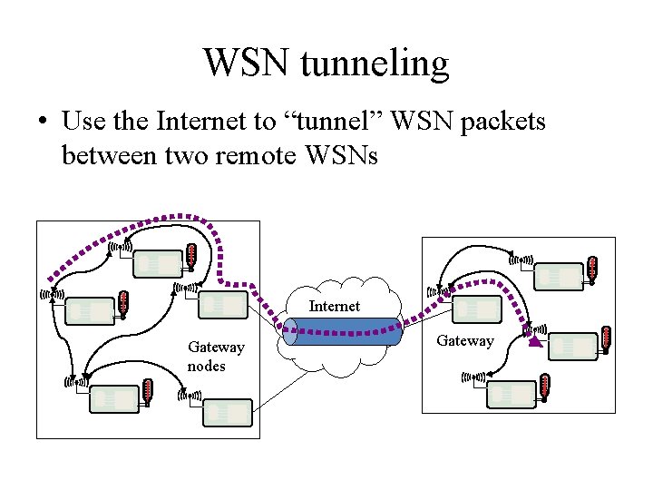
WSN tunneling • Use the Internet to “tunnel” WSN packets between two remote WSNs Internet Gateway nodes Gateway

Overview • • Principal options and difficulties Contention-based protocols Schedule-based protocols IEEE 802. 15. 4

Principal options and difficulties • Medium access in wireless networks is difficult mainly because of – Impossible (or very difficult) to sende and receive at the same time – Interference situation at receiver is what counts for transmission success, but can be very different from what sender can observe – High error rates (for signaling packets) compound the issues • Requirement – As usual: high throughput, low overhead, low error rates, … – Additionally: energy-efficient, handle switched off devices!

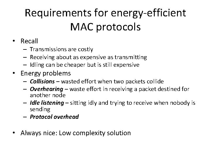
Requirements for energy-efficient MAC protocols • Recall – Transmissions are costly – Receiving about as expensive as transmitting – Idling can be cheaper but is still expensive • Energy problems – Collisions – wasted effort when two packets collide – Overhearing – waste effort in receiving a packet destined for another node – Idle listening – sitting idly and trying to receive when nobody is sending – Protocol overhead • Always nice: Low complexity solution

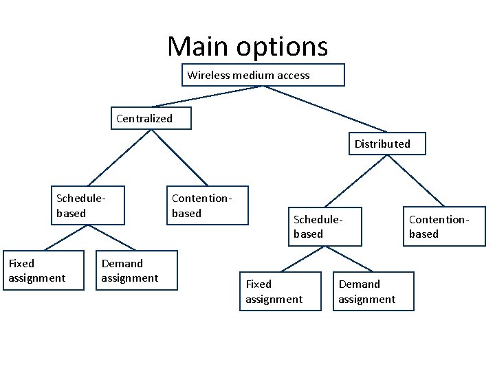
Main options Wireless medium access Centralized Distributed Schedulebased Fixed assignment Demand assignment Contentionbased

Centralized medium access • Idea: Have a central station control when a node may access the medium – Example: Polling, centralized computation of TDMA schedules – Advantage: Simple, quite efficient (e. g. , no collisions), burdens the central station • Not directly feasible for non-trivial wireless network sizes • But: Can be quite useful when network is somehow divided into smaller groups – Clusters, in each cluster medium access can be controlled centrally – compare Bluetooth piconets, for example ! Usually, distributed medium access is considered

Schedule- vs. contention-based MACs • Schedule-based MAC – A schedule exists, regulating which participant may use which resource at which time (TDMA component) – Typical resource: frequency band in a given physical space (with a given code, CDMA) – Schedule can be fixed or computed on demand • Usually: mixed – difference fixed/on demand is one of time scales – Usually, collisions, overhearing, idle listening no issues – Needed: time synchronization! • Contention-based protocols – Risk of colliding packets is deliberately taken – Hope: coordination overhead can be saved, resulting in overall improved efficiency – Mechanisms to handle/reduce probability/impact of collisions required – Usually, randomization used somehow

Overview • Principal options and difficulties • Contention-based protocols – MACA – S-MAC, T-MAC – Preamble sampling, B-MAC – PAMAS • Schedule-based protocols • IEEE 802. 15. 4

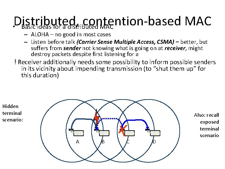
Distributed, contention-based MAC • Basic ideas for a distributed MAC – ALOHA – no good in most cases – Listen before talk (Carrier Sense Multiple Access, CSMA) – better, but suffers from sender not knowing what is going on at receiver, might destroy packets despite first listening for a ! Receiver additionally needs some possibility to inform possible senders in its vicinity about impending transmission (to “shut them up” for this duration) Hidden terminal scenario: A B C D Also: recall exposed terminal scenario

Main options to shut up senders • Receiver informs potential interferers while a reception is on-going – By sending out a signal indicating just that – Problem: Cannot use same channel on which actual reception takes place ! Use separate channel for signaling – Busy tone protocol • Receiver informs potential interferers before a reception is on-going – Can use same channel – Receiver itself needs to be informed, by sender, about impending transmission – Potential interferers need to be aware of such information, need to store it

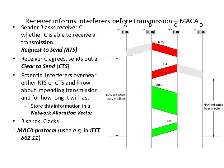
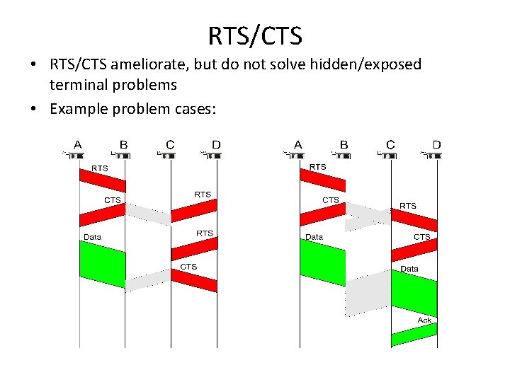
Receiver informs interferers before transmission – MACA • Sender B asks receiver C whether C is able to receive a transmission Request to Send (RTS) • Receiver C agrees, sends out a Clear to Send (CTS) • Potential interferers overhear either RTS or CTS and know about impending transmission and for how long it will last – Store this information in a Network Allocation Vector • B sends, C acks ! MACA protocol (used e. g. in IEEE 802. 11)

RTS/CTS • RTS/CTS ameliorate, but do not solve hidden/exposed terminal problems • Example problem cases:

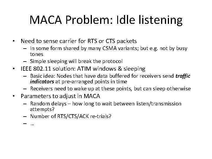
MACA Problem: Idle listening • Need to sense carrier for RTS or CTS packets – In some form shared by many CSMA variants; but e. g. not by busy tones – Simple sleeping will break the protocol • IEEE 802. 11 solution: ATIM windows & sleeping – Basic idea: Nodes that have data buffered for receivers send traffic indicators at pre-arranged points in time – Receivers need to wake up at these points, but can sleep otherwise • Parameters to adjust in MACA – Random delays – how long to wait between listen/transmission attempts? – Number of RTS/CTS/ACK re-trials? – …

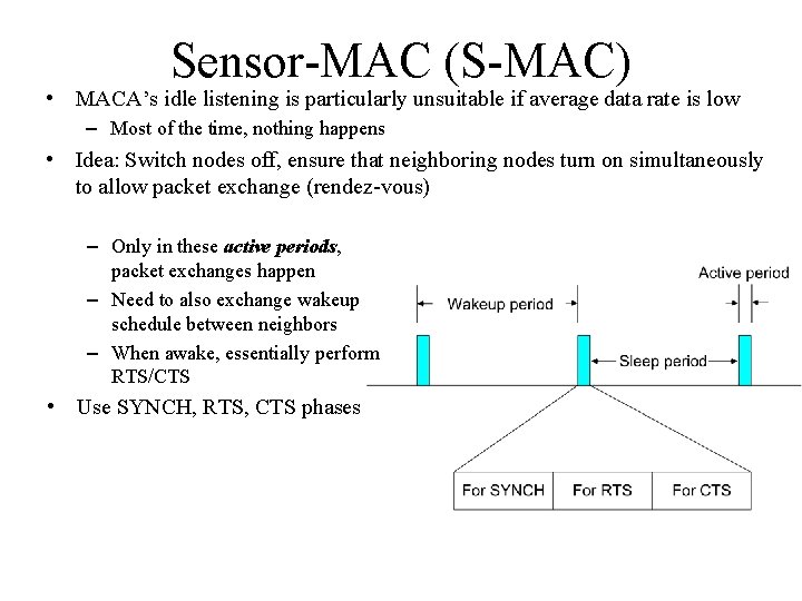
Sensor-MAC (S-MAC) • MACA’s idle listening is particularly unsuitable if average data rate is low – Most of the time, nothing happens • Idea: Switch nodes off, ensure that neighboring nodes turn on simultaneously to allow packet exchange (rendez-vous) – Only in these active periods, packet exchanges happen – Need to also exchange wakeup schedule between neighbors – When awake, essentially perform RTS/CTS • Use SYNCH, RTS, CTS phases

Sensor-MAC (S-MAC) • When competing for the medium, the nodes use the RTS/CTS handshake, including the virtual carrier-sense mechanism, whereby a node maintains a NAV variable. • The NAV mechanism can be readily used to switch off the node during ongoing transmissions to avoid overhearing. • If we can arrange that the schedules of node x and its neighbours are synchronized, node x and all its neighbours wake up at the same time and x can reach all of them with a single SYNCH packet. • The S-MAC protocol allows neighbouring nodes to agree on the same schedule and to create virtual clusters. • The clustering structure refers solely to the exchange of schedules; the transfer of data packets is not influenced by virtual clustering.

Sensor-MAC (S-MAC) • By this approach, a large multihop network is partitioned into “islands of schedule synchronization”. • Border nodes have to follow two or more different schedules for broadcasting their SYNCH packets and forwarding data packets. • Thus, they expend more energy than nodes only having neighbours of the same “schedule regime”. • The periodic wakeup scheme adopted by S-MAC allows nodes to spend much time in the sleep mode, but there is also a price to pay in terms of latency. • Without further modifications, the per-hop latency of S-MAC will be approximately equal to the sleep period on average when all nodes follow the same schedule. • The adaptive-listening scheme, which roughly halves the per-hop latency.

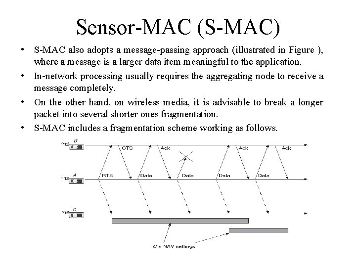
Sensor-MAC (S-MAC) • S-MAC also adopts a message-passing approach (illustrated in Figure ), where a message is a larger data item meaningful to the application. • In-network processing usually requires the aggregating node to receive a message completely. • On the other hand, on wireless media, it is advisable to break a longer packet into several shorter ones fragmentation. • S-MAC includes a fragmentation scheme working as follows.

Sensor-MAC (S-MAC) • This protocol is unfair because single nodes can block the medium for long time. • The fairness requirement has a different weight in a wireless sensor network than it has in a data network where users want to have fair medium access. • S-MAC has one major drawback: it is hard to adapt the length of the wakeup period to changing load situations, since this length is essentially fixed, as is the length of the listen period. • The T-MAC protocol is similar to S-MAC but adaptively shortens the listen period. • If a node x senses no activity on the medium for a specified duration, it is allowed to go back into sleep mode prematurely. • Therefore, if no node wants to transmit to x, the listen period can be ended quickly, whereas in S-MAC, the listen period has a fixed length.

The Mediation Device Protocol • The mediation device protocol is compatible with the peer-to-peer communication mode of the IEEE 802. 15. 4. • It allows each node in a WSN to go into sleep mode periodically and to wake up only for short times to receive packets from neighbour nodes. • There is no global time reference, each node has its own sleeping schedule, and does not take care of its neighbours sleep schedules. • Upon each periodic wakeup, a node transmits a short query beacon, indicating its node address and its willingness to accept packets from other nodes. • The node stays awake for some short time following the query beacon, to open up a window for incoming packets. • If no packet is received during this window, the node goes back into sleep mode.

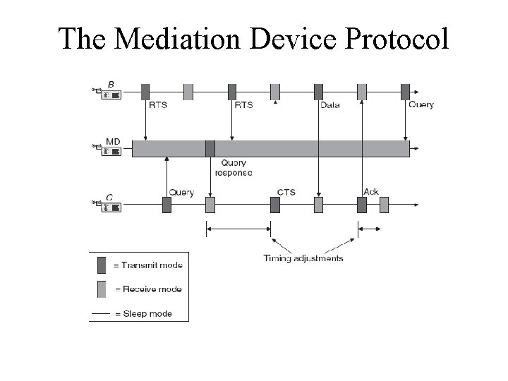
The Mediation Device Protocol • When a node wants to transmit a packet to a neighbour, it has to synchronize with it. • One option would be to have the sender actively waiting for query beacon, but this wastes considerable energy for synchronization purposes only. • The dynamic synchronization approach achieves this synchronization without requiring the transmitter to be awake permanently to detect the destinations query beacon. • To achieve this, a mediation device (MD) is used. • The mediation device is not energy constrained and can be active all the time; this scenario is illustrated in Figure. • Because of its full duty cycle, the mediation device can receive the query beacons from all nodes in its vicinity and learn their wakeup periods.

The Mediation Device Protocol

The Mediation Device Protocol • This protocol has some advantages. • First, it does not require any time synchronization between the nodes, only the mediation device has to learn the periods of the nodes. • Second, the protocol is asymmetric in the sense that most of the energy burden is shifted to the mediation device, which so far is assumed to be power unconstrained. • The other nodes can be in the sleep state most of the time and have to spend energy only for the periodic beacons. • Even when a transmitter wants to synchronize with the receiver, it does not have to wait actively for the query beacon, but can go back to sleep and wait for the mediation device to do the synchronization work. • This protocol has also some drawbacks: • The nodes transmit their query beacons without checking for ongoing transmissions and, thus, the beacons of different nodes may collide repeatedly when nodes have the same period and their wakeup periods overlap.

The Mediation Device Protocol • The mediation device is energy unconstrained, which does not confirm to the idea of a “simply thrown out” wireless sensor network. • There are sufficient mediation devices to cover all nodes. • The distributed mediation device protocol deals with these problems in a probabilistic manner. • It lets nodes randomly wake up and serve as MD for a certain time and afterward lets them go back to their regular periodic wakeup behaviour. • However, under these assumptions, it cannot be expected that a temporary MD knows all its neighbours' periods and wakeup times. • A problem with this approach is that nodes A and B may have two or more MD devices in their vicinity, causing a collision of several query responses.

Wakeup Radio Concepts • The ideal situation would be if a node were always in the receiving state when a packet is transmitted to it, in the transmitting state when it transmits a packet, and in the sleep state at all other times; the idle state should be avoided. • The wakeup radio concept strives to achieve this goal by a simple, “powerless” receiver that can trigger a main receiver if necessary. • One proposed wakeup MAC protocol assumes the presence of several parallel data channels, separated either in frequency (FDMA) or by choosing different codes in a CDMA schemes. • A node wishing to transmit a data packet randomly picks one of the channels and performs a carrier sensing operation. • If the channel is busy, the node makes another random channel choice and repeats the carrier-sensing operation. • After a certain number of unsuccessful trials, the node backs off for a random time and starts again.

Wakeup Radio Concepts • If the channel is idle, the node sends a wakeup signal to the intended receiver, indicating both the receiver identification and the channel to use. • The receiver wakes up its data transceiver, tunes to the indicated channel, and the data packet transmission can proceed. • Afterward, the receiver can switch its data transceiver back into sleep mode. • This wakeup radio concept has the significant advantage : • That only the low-power wakeup transceiver has to be switched on all the time while the much more energy consuming data transceiver is nonsleeping if and only if the node is involved in data transmissions. • This scheme is naturally traffic adaptive, that is, the MAC becomes more and more active as the traffic load increases. • Periodic wakeup schemes do not have this property.

Wakeup Radio Concepts • There also some drawbacks. • First, to our knowledge, there is no real hardware yet for such an ultralow power wakeup transceiver. • Second, the range of the wakeup radio and the data radio should be the same. • Third, this scheme critically relies on the wakeup channel’s ability to transport useful information like node addresses and channel identifications; this might not always be feasible. • If the wakeup channel does not support this feature, the transmitter wakes up all its neighbours when it emits a wakeup signal, creating an overhearing situation for most of them. • If the transmitting node is about to transmit a long data packet, it might be worthwhile to prepend the data packet with a short filter packet announcing the receiving node’s address. • All the other nodes can go back to sleep mode after receiving the filter packet.

Contention-based Protocols • In contention-based protocols, a given transmit opportunity toward a receiver node can in principle be taken by any of its neighbours. • If only one neighbour tries its luck, the packet goes through the channel. • If two or more neighbours try their luck, these have to compete with each other and in unlucky cases, for example, due to hidden-terminal situations, a collision might occur, wasting energy for both transmitter and receiver. • Two important contention based protocols are already discussed: (slotted) ALOHA and CSMA, along with mechanisms to solve the hiddenterminal problem. • In the following sections, we discuss variations of these protocols with the goal to conserve energy.

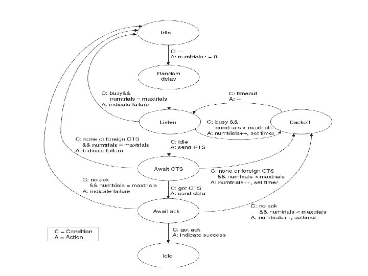
CSMA Protocols • Their are several CSMA variants for their inherent energy costs and their fairness, without specifying any measures for idle listening avoidance or overhearing avoidance. • Consider a multihop network with a single or only a few sinks and the same traffic pattern as already envisioned for STEM : A network that is idle for long times and starts to become active when triggered by an important external event. • Upon the triggering event, all nodes wish to transmit simultaneously, potentially creating lots of collisions. • In the case that the nodes want to send their packets periodically, the danger of collisions is repeated if no special measures are taken. • The nodes are assumed to know an upstream neighbour to which they have to forward packets destined for the sink. • This upstream neighbour is also called the parent node. • Each node generates local sensor traffic and additionally works as a forwarder for downstream nodes. Only a single channel is required.

CSMA Protocols

CSMA Protocols • Several variants of this skeleton (no random delay vs. random delay, random listening time vs. constant listening time, fixed window backoff vs. exponentially increasing backoff vs. Exponentially decreasing backoff vs. no backoff) have been investigated in a single-hop scenario with a triggering event. • It turns out that protocols with random delay, fixed listening time, and a backoff algorithm with sleeping radio transceiver give the best throughput as well as lowest aggregate energy consumption, when compared with other CSMA variants, including IEEE 802. 11.

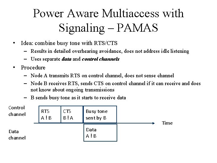
Power Aware Multiaccess with Signaling – PAMAS • Idea: combine busy tone with RTS/CTS – Results in detailed overhearing avoidance, does not address idle listening – Uses separate data and control channels • Procedure – Node A transmits RTS on control channel, does not sense channel – Node B receives RTS, sends CTS on control channel if it can receive and does not know about ongoing transmissions – B sends busy tone as it starts to receive data Control channel Data channel RTS A!B CTS B!A Busy tone sent by B Data A!B Time

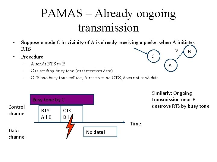
PAMAS – Already ongoing transmission • • Suppose a node C in vicinity of A is already receiving a packet when A initiates RTS ? B C Procedure – A sends RTS to B – C is sending busy tone (as it receives data) – CTS and busy tone collide, A receives no CTS, does not send data Similarly: Ongoing transmission near B destroys RTS by busy tone Busy tone by C Control channel RTS A!B CTS B!A Time Data channel A No data!

PAMAS • When can a node put its transceivers (control and data) into sleep mode? • Any time a node knows that it cannot transmit or receive packets because some other node in its vicinity is already doing so. • However, the decision to go into sleep mode raises an important question: when to wake up again? • This decision is easy if a node x knows about the length of an ongoing transmission, for example from overhearing the RTS or CTS packets or the header of the data packets on the data channel. • However, often this length is unknown to x, for example, because these packets are corrupted or a foreign data transmission cycle starts when x is just sleeping. • Additional procedures are needed to resolve this. • Suppose that x wakes up and finds the data channel busy. • There are two cases to distinguish: • either x has no own packet to send or x wants to transmit.

• • PAMAS In the first case, x desires to go back into sleep mode and to wake up exactly when the ongoing transmission ends to be able to receive an immediately following packet. Waking up at the earliest possible time has the advantage of avoiding unwanted delays. However, since x may not have overheard the RTS, CTS, or data packet header belonging to the ongoing transmission, it runs a probing protocol on the control channel to inquire the length of the ongoing packet. This probing protocol works similar to a binary search algorithm. In the other case, x wakes up during an ongoing transmission and wants to transmit a packet. Therefore, x has not only to take care of ongoing transmissions but also of ongoing receptions in its vicinity. To find the time for the next wakeup, x runs the described probing protocol for the set of transmitters, giving a time t when the longest ongoing transmission ends. In addition, x runs a similar probing protocol for the set of receivers in its neighborhood, indicating the time r when the longest ongoing reception ends.

Overview • Principal options and difficulties • Contention-based protocols • Schedule-based protocols – LEACH – SMACS – TRAMA • IEEE 802. 15. 4

Schedule-based Protocols • We discuss some schedule-based protocols that do not explicitly address idle listening avoidance but do so implicitly, for example, by employing TDMA schemes, which explicitly assign transmission and reception opportunities to nodes and let them sleep at all other times. • A second fundamental advantage of schedule-based protocols is that transmission schedules can be computed such that no collisions occur at receivers and hence no special mechanisms are needed to avoid hiddenterminal situations. • However, these schemes also have downsides. • First, the setup and maintenance of schedules involves signalling traffic, especially when faced to variable topologies. • Second, if a TDMA variant is employed, time is divided into comparably small slots, and both transmitter and receiver have to agree to slot boundaries to actually meet each other and to avoid overlaps with other slots, which would lead to collisions.

Schedule-based Protocols • A third drawback is that such schedules are not easily adapted to different load situations on small timescales. • Specifically, in TDMA, it is difficult for a node to give up unused time slots to its neighbours. • A further disadvantage is that the schedule of a node (and possibly those of its neighbours) may require a significant amount of memory, which is a scarce resource in several sensor node designs. • Finally, distributed assignment of conflict-free TDMA schedules is a difficult problem in itself.

Low-Energy Adaptive Clustering Hierarchy (LEACH) • The LEACH protocol assumes a dense sensor network of homogeneous, energy-constrained nodes, which shall report their data to a sink node. • In LEACH, a TDMA-based MAC protocol is integrated with clustering and a simple “routing” protocol. • LEACH partitions the nodes into clusters and in each cluster a dedicated node, the clusterhead, is responsible for creating and maintaining a TDMA schedule; all the other nodes of a cluster are member nodes. • To all member nodes, TDMA slots are assigned, which can be used to exchange data between the member and the clusterhead; there is no peer-topeer communication. • With the exception of their time slots, the members can spend their time in sleep state. • The clusterhead aggregates the data of its members and transmits it to the sink node or to other nodes for further relaying. • Since the sink is often far away, the clusterhead must spend significant energy for this transmission. • The clusterheads role is energy consuming since it is always switched on and is responsible for the long-range transmissions.

Low-Energy Adaptive Clustering Hierarchy (LEACH) • After the clusters have been formed, each clusterhead picks a random CDMA code for its cluster, which it broadcasts and which its member nodes have to use subsequently. • A critical network parameter is the percentage of nodes that are clusterheads. • If there are only a few clusterheads, the expected distance between a member node and its clusterhead becomes longer and therefore the member has to spend more energy to reach its clusterhead. • On the other hand, if there are many clusterheads, there will be more energy expensive transmissions from clusterheads to the sink and less aggregation. • Therefore, there exists an optimum percentage of clusterheads, which for the scenario investigated is ≈5%. • If this optimum is chosen, more energy is conserved. • In addition, since LEACH distributes the clusterhead role fairly to all nodes, they tend to die at about the same time.

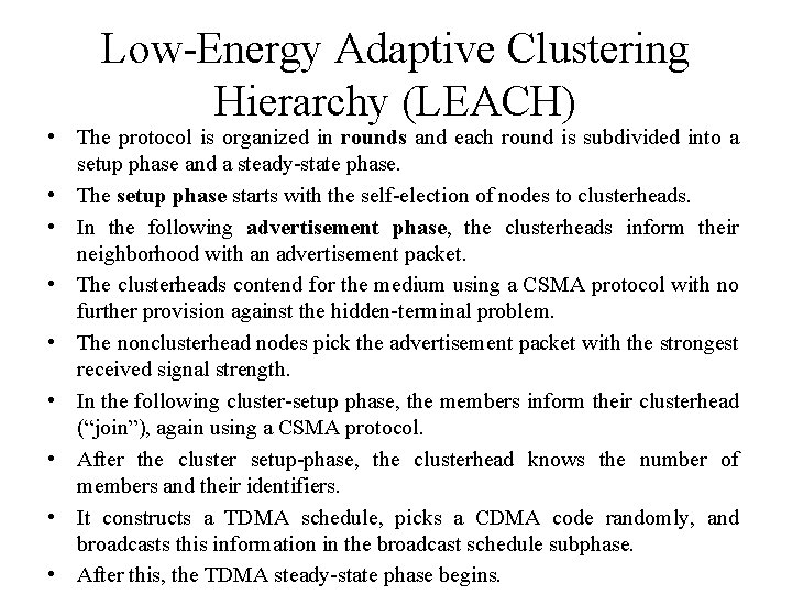
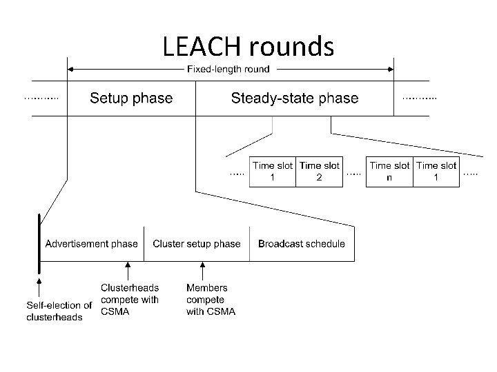
Low-Energy Adaptive Clustering Hierarchy (LEACH) • The protocol is organized in rounds and each round is subdivided into a setup phase and a steady-state phase. • The setup phase starts with the self-election of nodes to clusterheads. • In the following advertisement phase, the clusterheads inform their neighborhood with an advertisement packet. • The clusterheads contend for the medium using a CSMA protocol with no further provision against the hidden-terminal problem. • The nonclusterhead nodes pick the advertisement packet with the strongest received signal strength. • In the following cluster-setup phase, the members inform their clusterhead (“join”), again using a CSMA protocol. • After the cluster setup-phase, the clusterhead knows the number of members and their identifiers. • It constructs a TDMA schedule, picks a CDMA code randomly, and broadcasts this information in the broadcast schedule subphase. • After this, the TDMA steady-state phase begins.

LEACH rounds

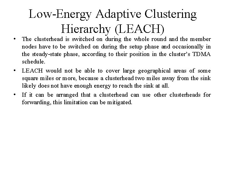
Low-Energy Adaptive Clustering Hierarchy (LEACH) • The clusterhead is switched on during the whole round and the member nodes have to be switched on during the setup phase and occasionally in the steady-state phase, according to their position in the cluster’s TDMA schedule. • LEACH would not be able to cover large geographical areas of some square miles or more, because a clusterhead two miles away from the sink likely does not have enough energy to reach the sink at all. • If it can be arranged that a clusterhead can use other clusterheads forwarding, this limitation can be mitigated.

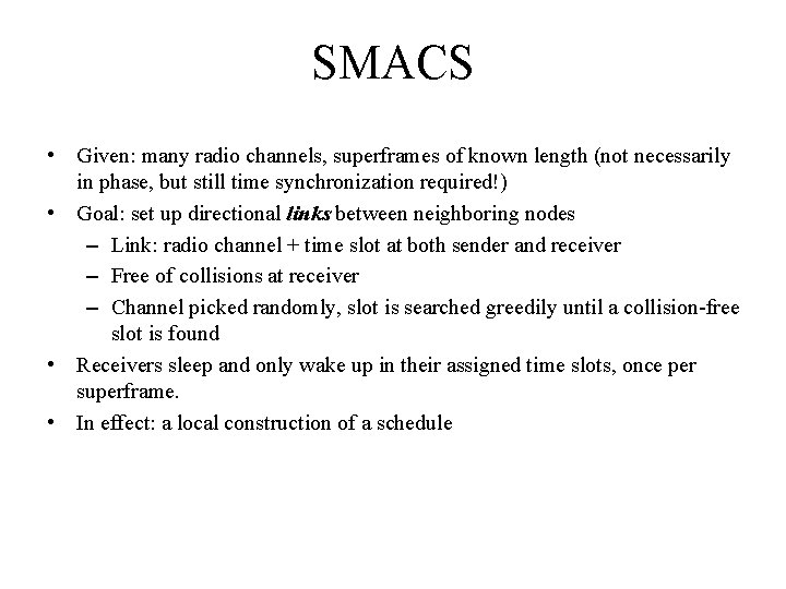
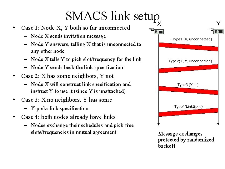
SMACS • Given: many radio channels, superframes of known length (not necessarily in phase, but still time synchronization required!) • Goal: set up directional links between neighboring nodes – Link: radio channel + time slot at both sender and receiver – Free of collisions at receiver – Channel picked randomly, slot is searched greedily until a collision-free slot is found • Receivers sleep and only wake up in their assigned time slots, once per superframe. • In effect: a local construction of a schedule

SMACS link setup • Case 1: Node X, Y both so far unconnected – Node X sends invitation message – Node Y answers, telling X that is unconnected to any other node – Node X tells Y to pick slot/frequency for the link – Node Y sends back the link specification • Case 2: X has some neighbors, Y not – Node X will construct link specification and instruct Y to use it (since Y is unattached) • Case 3: X no neighbors, Y has some – Y picks link specification • Case 4: both nodes already have links – Nodes exchange their schedules and pick free slots/frequencies in mutual agreement Message exchanges protected by randomized backoff

SMACS • This protocol allows to set up static connections between stationary nodes. • Since the neighborhood discovery process is repeated from time to time, the protocol can adapt to changes in topology. • A critical issue with this protocol is the choice of the superframe length. • It should be large enough to accommodate the highest node degree in the network, which is a random variable for random deployments. • If the superframe length is too short, some of a node’s neighbors may simply not be visible to it. • A second problem occurs in a densely populated sensor network with low traffic load, where schedules are highly populated and nodes wake up quite often just to notice that there is no packet destined to them. • The number of wakeup slots depends on the node density for this protocol.

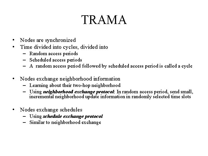
TRAMA • Nodes are synchronized • Time divided into cycles, divided into – Random access periods – Scheduled access periods – A random access period followed by scheduled access period is called a cycle • Nodes exchange neighborhood information – Learning about their two-hop neighborhood – Using neighborhood exchange protocol: In random access period, send small, incremental neighborhood update information in randomly selected time slots • Nodes exchange schedules – Using schedule exchange protocol – Similar to neighborhood exchange

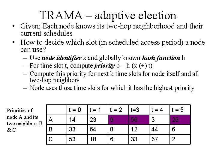
TRAMA – adaptive election • Given: Each node knows its two-hop neighborhood and their current schedules • How to decide which slot (in scheduled access period) a node can use? – Use node identifier x and globally known hash function h – For time slot t, compute priority p = h (x (+) t) – Compute this priority for next k time slots for node itself and all two-hop neighbors – Node uses those time slots for which it has the highest priority Priorities of node A and its two neighbors B &C t=0 t=1 t=2 t=3 t=4 t=5 A 14 23 9 56 3 26 B 33 64 8 12 44 6 C 53 18 6 33 57 2

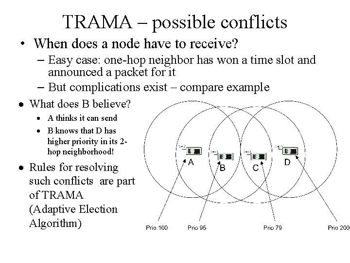
TRAMA – possible conflicts • When does a node have to receive? – Easy case: one-hop neighbor has won a time slot and announced a packet for it – But complications exist – compare example · What does B believe? · A thinks it can send · B knows that D has higher priority in its 2 hop neighborhood! · Rules for resolving such conflicts are part of TRAMA (Adaptive Election Algorithm)

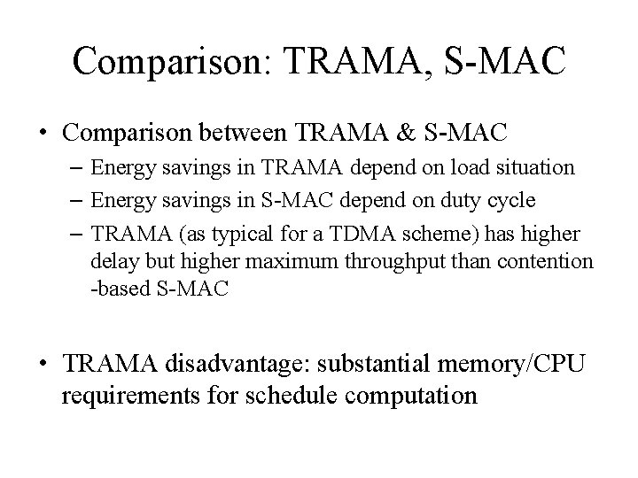
Comparison: TRAMA, S-MAC • Comparison between TRAMA & S-MAC – Energy savings in TRAMA depend on load situation – Energy savings in S-MAC depend on duty cycle – TRAMA (as typical for a TDMA scheme) has higher delay but higher maximum throughput than contention -based S-MAC • TRAMA disadvantage: substantial memory/CPU requirements for schedule computation

Overview • • Principal options and difficulties Contention-based protocols Schedule-based protocols IEEE 802. 15. 4

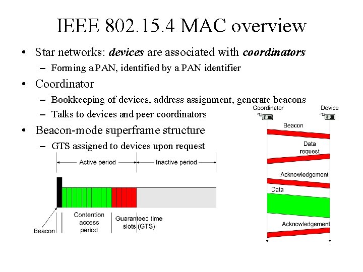
IEEE 802. 15. 4 • IEEE standard for low-rate WPAN applications • Goals: low-to-medium bit rates, moderate delays without too stringent guarantee requirements, low energy consumption • Physical layer – 20 kbps over 1 channel @ 868 -868. 6 MHz – 40 kbps over 10 channels @ 905 – 928 MHz – 250 kbps over 16 channels @ 2. 4 GHz • MAC protocol – Single channel at any one time – Combines contention-based and schedule-based schemes – Asymmetric: nodes can assume different roles

IEEE 802. 15. 4 MAC overview • Star networks: devices are associated with coordinators – Forming a PAN, identified by a PAN identifier • Coordinator – Bookkeeping of devices, address assignment, generate beacons – Talks to devices and peer coordinators • Beacon-mode superframe structure – GTS assigned to devices upon request