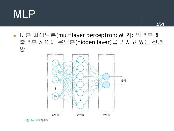
761 l current input for each layer in

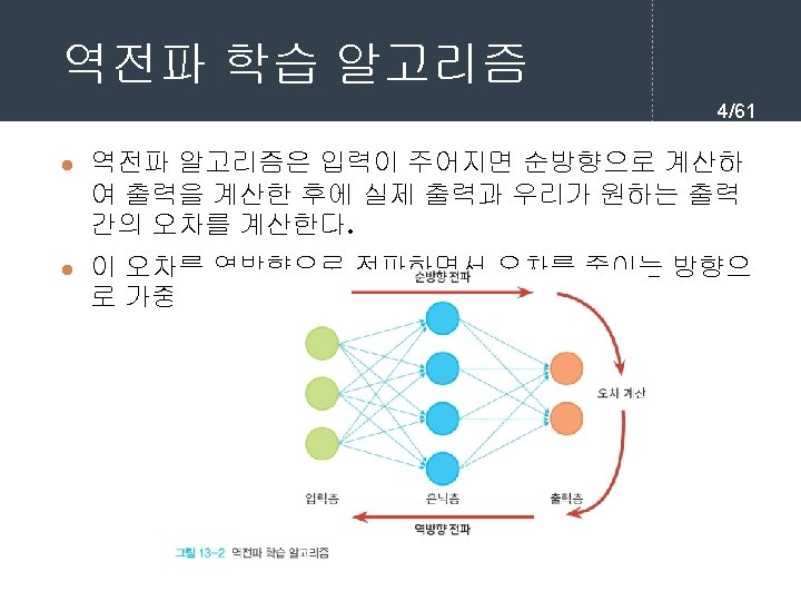
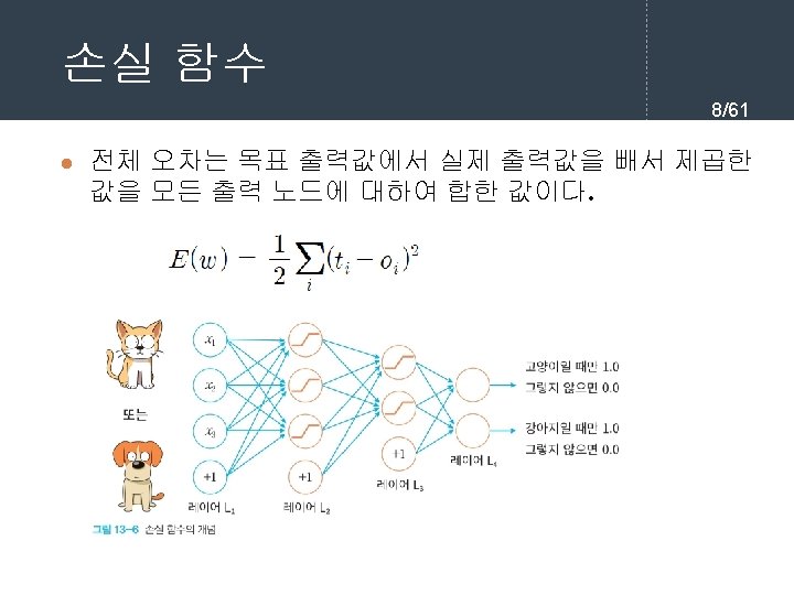
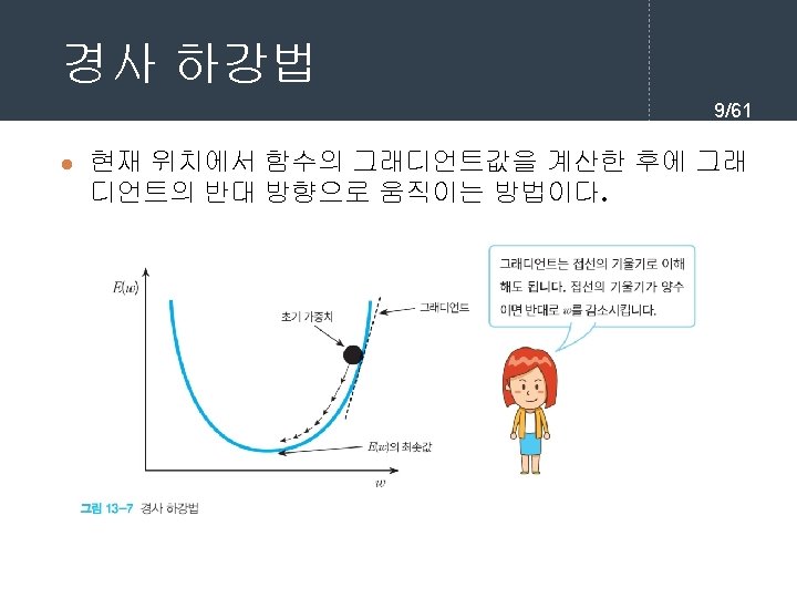
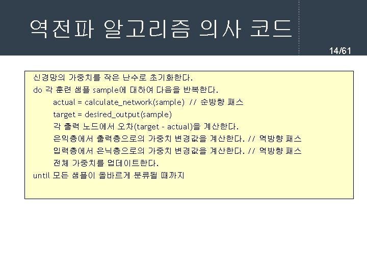
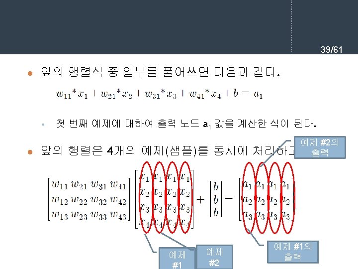
역전파 학습 알고리즘 7/61 l 순방향 출력 계산 current = input for each layer in network for each neuron i in layer net = get_sum(weights[i], current) # 입력의 가중합을 계산 output[i] = activation_func(net) # 각 노드들의 출력을 계산한다. current = output # 다음 계층은 현재 계층의 출력을 입력으로 사용한다.

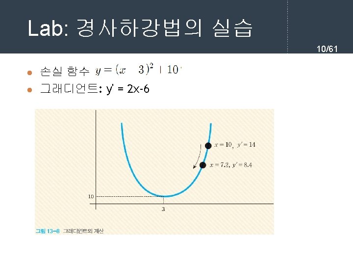
경사 하강법 프로그래밍 11/61 x = 10 learning_rate = 0. 01 precision = 0. 00001 max_iterations = 100 # 손실 함수를 람다식으로 정의한다. loss_func = lambda x: (x-3)**2 + 10 # 그래디언트를 람다식으로 정의한다. 손실 함수의 1차 미분값이다. gradient = lambda x: 2*x-6 # 그래디언트 강하법 for i in range(max_iterations): x = x - learning_rate * gradient(x) print("손실 함수값(", x, ")=", loss_func(x)) print("최소값 = ", x)

실행 결과 12/61. . . 손실 함수값( 4. 02701132062644 )= 11. 054752252694865 손실 함수값( 4. 006471094213911 )= 11. 012984063488148 손실 함수값( 3. 9863416723296328 )= 10. 972869894574016 손실 함수값( 3. 9666148388830402 )= 10. 934344246748886 손실 함수값( 3. 947282542105379 )= 10. 897344214577629 손실 함수값( 3. 9283368912632715 )= 10. 861809383680356 최소값 = 3. 9283368912632715

Lab: 역전파 알고리즘 시뮬레이 션 22/61 l http: //www. emergentmind. com/neural-network

실행결과 43/61 [[0. 02391914] [0. 9757925 ] [0. 97343127] [0. 03041428]]

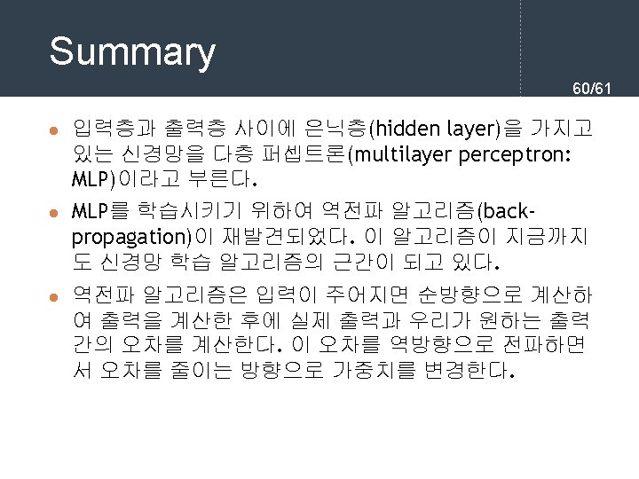
모델 작성 49/61 from tf. keras. models import Sequential model = Sequential() from tf. keras. layers import Dense model. add(Dense(units=64, activation='sigmoid', input_dim=100)) # ① model. add(Dense(units=10, activation='sigmoid')) #②

학습 과정 정의 50/61 model. compile(loss='mse', optimizer='sgd', metrics=['accuracy']) model. fit(X, y, epochs=5, batch_size=32) 학습 loss_and_metrics = model. evaluate(X, y, batch_size=128) classes = model. predict(new_X, batch_size=128) 평가와 예측

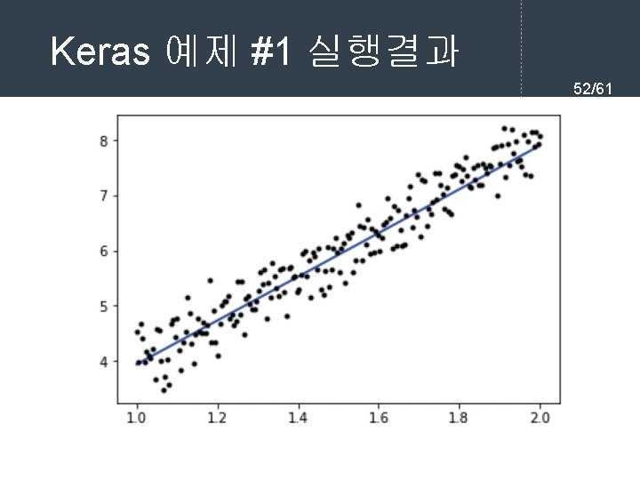
Keras 예제 #1 선형 회귀 51/61 import tensorflow as tf import numpy as np import matplotlib. pyplot as plt # 가상적인 데이터 생성 X = data = np. linspace(1, 2, 200) # 시작값=1, 종료값=2, 개수=200 y = x*4 + np. random. randn(200) * 0. 3 # x를 4배로 하고 편차 0. 3정도의 가우시안 잡음 추가 model = tf. keras. models. Sequential() model. add(tf. keras. layers. Dense(1, input_dim=1, activation='linear')) model. compile(optimizer='sgd', loss='mse', metrics=['mse']) model. fit(X, y, batch_size=1, epochs=30) predict = model. predict(data) plt. plot(data, predict, 'b', data, y, 'k. ') # 첫 번째 그래프는 파란색 마커로 plt. show() # 두 번째 그래프는 검정색. 으로 그린다.

Keras 예제 #2 XOR 53/61 import tensorflow as tf import numpy as np X = np. array([[0, 0], [0, 1], [1, 0], [1, 1]]) y = np. array([[0], [1], [0]]) model = tf. keras. models. Sequential() model. add(tf. keras. layers. Dense(2, input_dim=2, activation='sigmoid')) model. add(tf. keras. layers. Dense(1, activation='sigmoid')) sgd = tf. keras. optimizers. SGD(lr=0. 1) model. compile(loss='mean_squared_error', optimizer=sgd) model. fit(X, y, batch_size=1, epochs=1000) print(model. predict(X))

Keras 예제 #2 실행결과 54/61 [[0. 19608304] [0. 64313614] [0. 6822454 ] [0. 53627 ]] [[0. 02743807] [0. 9702845 ] [0. 9704155 ] [0. 03712982]] 반복횟수(에포크) 를 10000으로 늘 린다면

Lab: MLP를 사용한 MNIST 숫자 인식 55/61

Lab: MLP를 사용한 MNIST 숫자 인식 56/61 import tensorflow as tf batch_size = 128 # 가중치를 변경하기 전에 처리하는 샘플의 개수 num_classes = 10 # 출력 클래스의 개수 epochs = 20 # 에포크의 개수 # 데이터를 학습 데이터와 테스트 데이터로 나눈다. (x_train, y_train), (x_test, y_test) = tf. keras. datasets. mnist. load_data() # 입력 이미지를 2차원에서 1차원 벡터로 변경한다. x_train = x_train. reshape(60000, 784) x_test = x_test. reshape(10000, 784) # 입력 이미지의 픽셀 값이 0. 0에서 1. 0 사이의 값이 되게 한다. x_train = x_train. astype('float 32') x_test = x_test. astype('float 32') x_train /= 255 x_test /= 255

Lab: MLP를 사용한 MNIST 숫자 인식 57/61 # 클래스의 개수에 따라서 하나의 출력 픽셀만이 1이 되게 한다. # 예를 들면 1 0 0 0 0 0과 같다. y_train = tf. keras. utils. to_categorical(y_train, num_classes) y_test = tf. keras. utils. to_categorical(y_test, num_classes) # 신경망의 모델을 구축한다. model = tf. keras. models. Sequential() model. add(tf. keras. layers. Dense(512, activation='sigmoid', input_shape=(784, ))) model. add(tf. keras. layers. Dense(num_classes, activation='sigmoid')) model. summary() sgd = tf. keras. optimizers. SGD(lr=0. 1)

Lab: MLP를 사용한 MNIST 숫자 인식 58/61 # 손실 함수를 제곱 오차 함수로 설정하고 학습 알고리즘은 SGD 방식으로 한다. model. compile(loss='mean_squared_error', optimizer=sgd, metrics=['accuracy']) # 학습을 수행한다. history = model. fit(x_train, y_train, batch_size=batch_size, epochs=epochs) # 학습을 평가한다. score = model. evaluate(x_test, y_test, verbose=0) print('테스트 손실값: ', score[0]) print('테스트 정확도: ', score[1])

실행결과 59/61 _________________________________ Layer (type) Output Shape Param # ================================= dense_4 (Dense) (None, 512) 401920 _________________________________ dense_5 (Dense) (None, 10) 5130 ================================= Total params: 407, 050 Trainable params: 407, 050 Non-trainable params: 0. . . Epoch 18/20 60000/60000 [===============] - 1 s 18 us/sample - loss: 0. 0344 acc: 0. 8480 Epoch 19/20 60000/60000 [===============] - 1 s 18 us/sample - loss: 0. 0335 acc: 0. 8505 Epoch 20/20 60000/60000 [===============] - 1 s 18 us/sample - loss: 0. 0328 acc: 0. 8530 테스트 손실값: 0. 03148304631710053 테스트 정확도: 0. 8628

Q&A 61/61