405 ECONOMETRICS Chapter 11 HETEROSCEDASTICITY WHAT HAPPENS IF

405 ECONOMETRICS Chapter # 11: HETEROSCEDASTICITY: WHAT HAPPENS IF THE ERROR VARIANCE IS NONCONSTANT? Domodar N. Gujarati Prof. M. El-Sakka Dept of Economics Kuwait University

• • • As in Chapter 10, we seek answers to the following questions: 1. What is the nature of heteroscedasticity? 2. What are its consequences? 3. How does one detect it? 4. What are the remedial measures?

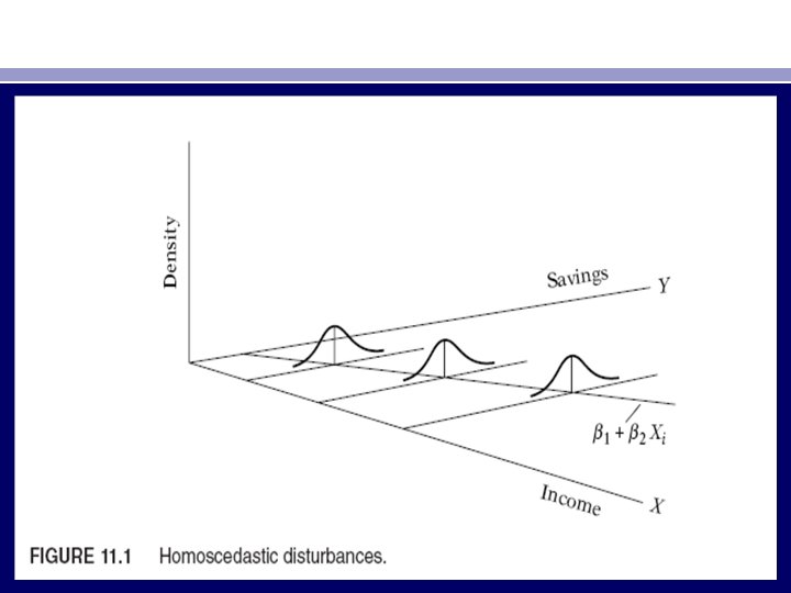
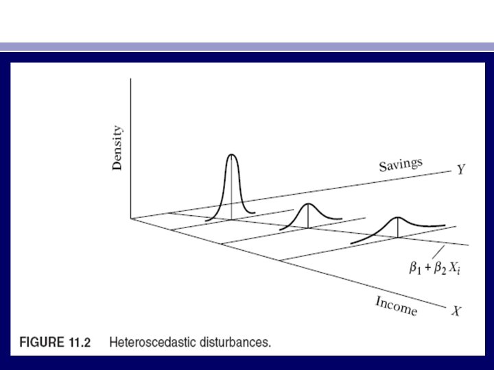
THE NATURE OF HETEROSCEDASTICITY • One of the important assumptions of the classical linear regression model is that the variance of each disturbance term ui, conditional on the chosen values of the explanatory variables, is some constant number equal to σ2. This is the assumption of homoscedasticity, or equal (homo) spread (scedasticity), that is, equal variance. Symbolically, • Eu 2 i = σ2 i = 1, 2, . . . , n (11. 1. 1) • Look at Figure 11. 1. In contrast, consider Figure 11. 2, the variances of Yi are not the same. Hence, there is heteroscedasticity. Symbolically, • Eu 2 i = σ2 i (11. 1. 2) • Notice the subscript of σ2, which reminds us that the conditional variances of ui (= conditional variances of Yi) are no longer constant.

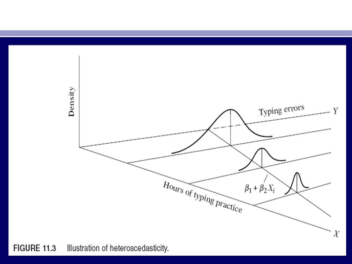
• Assume that in the two-variable model Yi = β 1 + β 2 Xi + ui , Y represents savings and X represents income. Figures 11. 1 and 11. 2 show that as income increases, savings on the average also increase. But in Figure 11. 1 the variance of savings remains the same at all levels of income, whereas in Figure 11. 2 it increases with income. It seems that in Figure 11. 2 the higher income families on the average save more than the lower-income families, but there is also more variability in their savings. • There are several reasons why the variances of ui may be variable, some of which are as follows. • 1. Following the error-learning models, as people learn, their errors of behavior become smaller over time. In this case, σ2 i is expected to decrease. As an example, consider Figure 11. 3, which relates the number of typing errors made in a given time period on a test to the hours put in typing practice.

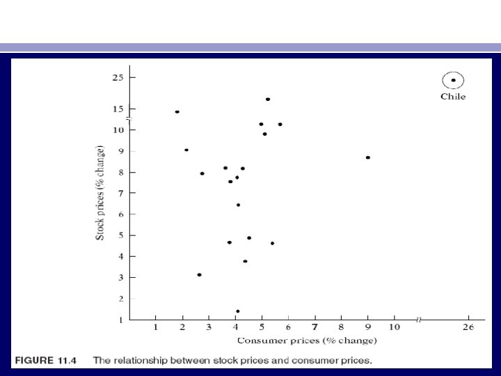
• 2. As incomes grow, people have more discretionary income and hence more scope for choice about the disposition of their income. Hence, σ2 i is likely to increase with income. Similarly, companies with larger profits are generally expected to show greater variability in their dividend policies than companies with lower profits. • 3. As data collecting techniques improve, σ2 i is likely to decrease. Thus, banks that have sophisticated data processing equipment are likely to commit fewer errors in the monthly or quarterly statements of their customers than banks without such facilities. • 4. Heteroscedasticity can also arise as a result of the presence of outliers, (either very small or very large) in relation to the observations in the sample Figure 11. 4. The inclusion or exclusion of such an observation, especially if the sample size is small, can substantially alter the results of regression analysis. Chile can be regarded as an outlier because the given Y and X values are much larger than for the rest of the countries. In situations such as this, it would be hard to maintain the assumption of homoscedasticity.

• 5. Another source of heteroscedasticity arises from violating Assumption 9 of CLRM, namely, that the regression model is correctly specified, very often what looks like heteroscedasticity may be due to the fact that some important variables are omitted from the model. But if the omitted variables are included in the model, that impression may disappear. • 6. Another source of heteroscedasticity is skewness in the distribution of one or more regressors included in the model. Examples are economic variables such as income, wealth, and education. It is well known that the distribution of income and wealth in most societies is uneven, with the bulk of the income and wealth being owned by a few at the top. • 7. Other sources of heteroscedasticity: As David Hendry notes, heteroscedasticity can also arise because of – (1) incorrect data transformation (e. g. , ratio or first difference transformations) – (2) incorrect functional form (e. g. , linear versus log–linear models).

• Note that the problem of heteroscedasticity is likely to be more common in cross-sectional than in time series data. In cross-sectional data, members may be of different sizes, such as small, medium, or large firms or low, medium, or high income. In time series data, on the other hand, the variables tend to be of similar orders of magnitude. Examples are GNP, consumption expenditure, savings.

THE METHOD OF GENERALIZED LEAST SQUARES (GLS( • If ui is hetroschedastic βˆ2 is no longer best, although it is still unbiased. Intuitively, we can see the reason from Table 11. 1. As the table shows, there is considerable variability in the earnings between employment classes. If we were to regress per-employee compensation on the size of employment, we would like to make use of the knowledge that there is considerable interclass variability in earnings. Ideally, we would like to devise the estimating scheme in such a manner that observations coming from populations with greater variability are given less weight than those coming from populations with smaller variability. Examining Table 11. 1, we would like to weight observations coming from employment classes 10– 19 and 20– 49 more heavily than those coming from employment classes like 5– 9 and 250– 499, for the former are more closely clustered around their mean values than the latter, thereby enabling us to estimate the PRF more accurately.

• Unfortunately, the usual OLS method does not follow this strategy, but a method of estimation, known as generalized least squares (GLS), takes such information into account explicitly and is therefore capable of producing estimators that are BLUE. To see how this is accomplished, let us continue with the now-familiar two-variable model: • Y i = β 1 + β 2 X i + ui (11. 3. 1) • which for ease of algebraic manipulation we write as • Yi = β 1 X 0 i + β 2 Xi + ui (11. 3. 2) • where X 0 i = 1 for each i. Now assume that the heteroscedastic variances σ2 i are known. Divide through by σi to obtain: • which for ease of exposition we write as • Y*i = β*1 X*0 i + β*2 X*i + u*i (11. 3. 4)

• where the starred, . We use the notation β∗ 1 and β∗ 2, the parameters of the transformed model, to distinguish them from the usual OLS parameters β 1 and β 2. What is the purpose of transforming the original model? To see this, notice the following feature of the transformed error term: • which is a constant. That is, the variance of the transformed disturbance term u*i is now homoscedastic.

• The finding that it is u* that is homoscedastic suggests that if we apply OLS to the transformed model (11. 3. 3) it will produce estimators that are BLUE. This procedure of transforming the original variables in such a way that the transformed variables satisfy the assumptions of the classical model and then applying OLS to them is known as the method of generalized least squares (GLS). In short, GLS is OLS on the transformed variables that satisfy the standard least-squares assumptions. The estimators thus obtained are known as GLS estimators, and it is these estimators that are BLUE.

• The actual mechanics of estimating β*1 and β*2 are as follows. First, we write down the SRF of (11. 3. 3) • Yi/σi = βˆ*1 X 0 i/σi + βˆ*2 Xi/σi + uˆi/σi • or • Y*i = βˆ*1 X*0 i + βˆ*2 X*i + uˆ*i (11. 3. 6) • Now, to obtain the GLS estimators, we minimize • Σuˆ2*i = Σ(Y*i − βˆ*1 X*0 i − β*2 X*i )2 • that is, • The actual mechanics of minimizing (11. 3. 7) follow the standard calculus techniques the GLS estimator of β*2 is

• and its variance is given by • where wi = 1/σ2 i.

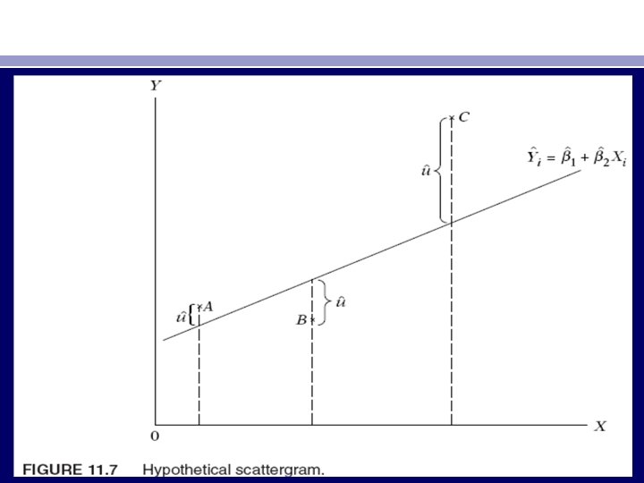
• • • The Difference between OLS and GLS Recall from Chapter 3 that in OLS we minimize: Σuˆ2 i =Σ(Yi − βˆ1 − βˆ2 Xi)2 (11. 3. 10) but in GLS we minimize the expression (11. 3. 7), which can also be written as Σwiuˆ2 i = Σwi(Yi − βˆ*1 X 0 i − βˆ*2 Xi)2 (11. 3. 11) where wi = 1/σ2 i Thus, in GLS we minimize a weighted sum of residual squares with wi = 1/σ2 i acting as the weights, but in OLS we minimize an unweighted or (what amounts to the same thing) equally weighted RSS. As (11. 3. 7) shows, in GLS the weight assigned to each observation is inversely proportional to its σi , that is, observations coming from a population with larger σi will get relatively smaller weight and those from a population with smaller σi will get proportionately larger weight in minimizing the RSS (11. 3. 11). To see the difference between OLS and GLS clearly, consider the hypothetical scattergram given in Figure 11. 7.

• In the (unweighted) OLS, each uˆ2 i associated with points A, B, and C will receive the same weight in minimizing the RSS. Obviously, in this case the uˆ2 i associated with point C will dominate the RSS. But in GLS the extreme observation C will get relatively smaller weight than the other two observations. • Since (11. 3. 11) minimizes a weighted RSS, it is appropriately known as weighted least squares (WLS), and the estimators thus obtained and given in (11. 3. 8) and (11. 3. 9) are known as WLS estimators. But WLS is just a special case of the more general estimating technique, GLS. In the context of heteroscedasticity, one can treat the two terms WLS and GLS interchangeably.

CONSEQUENCES OF USING OLS IN THE PRESENCE OF HETEROSCEDASTICITY • As we have seen, both βˆ*2 and βˆ2 are (linear) unbiased estimators: In repeated sampling, on the average, βˆ*2 and βˆ2 will equal the true β 2; that is, they are both unbiased estimators. But we know that it is βˆ*2 that is efficient, that is, has the smallest variance. What happens to our confidence interval, hypotheses testing, and other procedures if we continue to use the OLS estimator βˆ2? We distinguish two cases. • OLS Estimation Allowing for Heteroscedasticity • Suppose we use βˆ2 and use the variance formula given in (11. 2. 2), which takes into account heteroscedasticity explicitly. Using this variance, and assuming σ2 i are known, can we establish confidence intervals and test hypotheses with the usual t and F tests? The answer generally is no because it can be shown that var (βˆ*2) ≤ var (βˆ2), which means that confidence intervals based on the latter will be unnecessarily larger. As a result, the t and F tests are likely to give us inaccurate results.

• OLS Estimation Disregarding Heteroscedasticity • The situation can become serious if we not only use βˆ2 but also continue to use the usual (homoscedastic) variance formula given in (11. 2. 3) even if heteroscedasticity is present or suspected, whatever conclusions we draw or inferences we make may be very misleading.

DETECTION OF HETEROSCEDASTICITY • In most cases involving econometric investigations, heteroscedasticity may be a matter of intuition, educated guesswork, prior empirical experience, or sheer speculation. Some of the informal and formal methods are used for detecting heteroscedasticity. Most of these methods are based on the examination of the OLS residuals uˆi since they are the ones we observe, and not the disturbances ui. One hopes that they are good estimates of ui, a hope that may be fulfilled if the sample size is fairly large. • Informal Methods • Nature of the Problem. Very often the nature of the problem under consideration suggests whether heteroscedasticity is likely to be encountered. In cross-sectional data involving heterogeneous units, heteroscedasticity may be the rule rather than the exception. Thus, in a cross-sectional analysis involving the investment expenditure in relation to sales, rate of interest, etc. , heteroscedasticity is generally expected if small-, medium-, and largesize firms are sampled together.

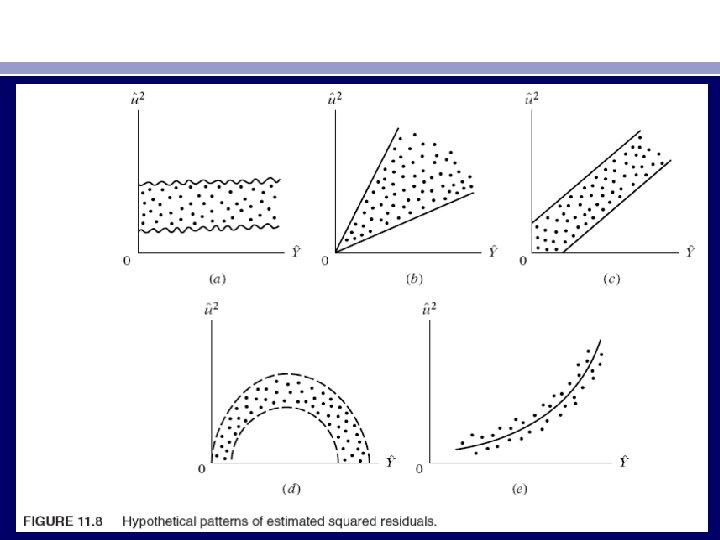
• Graphical Method • If there is no a priori or empirical information about the nature of heteroscedasticity, in practice one can do the regression analysis on the assumption that there is no heteroscedasticity and then do an examination of the residual squared uˆ2 i to see if they exhibit any systematic pattern. • Although uˆ2 i are not the same thing as u 2 i , they can be used as proxies especially if the sample size is sufficiently large. An examination of the uˆ2 i may reveal patterns such as those shown in Figure 11. 8. In Figure 11. 8 a we see that there is no systematic pattern between the two variables, suggesting that perhaps no heteroscedasticity is present in the data. Figure 11. 8 b to e, however, exhibits definite patterns. For instance, Figure 11. 8 c suggests a linear relationship, whereas Figure 11. 8 d and e indicates a quadratic relationship between uˆ2 i and Yˆi. Using such knowledge, albeit informal, one may transform the data in such a manner that the transformed data do not exhibit heteroscedasticity.

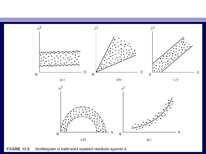
• Instead of plotting uˆ2 i against Yˆi, one may plot them against one of the explanatory variables Xi. • A pattern such as that shown in Figure 11. 9 c, for instance, suggests that the variance of the disturbance term is linearly related to the X variable. Thus, if in the regression of savings on income one finds a pattern such as that shown in Figure 11. 9 c, it suggests that the heteroscedastic variance may be proportional to the value of the income variable. This knowledge may help us in transforming our data in such a manner that in the regression on the transformed data the variance of the disturbance is homoscedastic.

• Formal Methods • Park Test. Park suggests that σ2 i is some function of the explanatory variable Xi. The functional form he suggested was • σ2 i = σ2 Xβi evi • or • ln σ2 i = ln σ2 + β ln Xi + vi (11. 5. 1) • where vi is the stochastic disturbance term. Since σ2 i is generally not known, Park suggests using uˆ2 i as a proxy and running the following regression: • ln uˆ2 i = ln σ2 + β ln Xi + vi = α + β ln Xi + vi (11. 5. 2) • If β turns out to be statistically significant, it would suggest that heteroscedasticity is present in the data. If it turns out to be insignificant, we may accept the assumption of homoscedasticity. The Park test is a two stage procedure. In the first stage we run the OLS regression disregarding the heteroscedasticity question. We obtain uˆi from this regression, and then in the second stage we run the regression (11. 5. 2).

• Although empirically appealing, the Park test has some problems. Goldfeld and Quandt have argued that the error term vi entering into (11. 5. 2) may not satisfy the OLS assumptions and may itself be heteroscedastic. • EXAMPLE 11. 1 Relationship between compensation and productivity • use the data given in Table 11. 1 to run the following regression: • Y i = β 1 + β 2 X i + ui • where Y = average compensation in thousands of dollars, X = average productivity in thousands of dollars, and i = ith employment size of the establishment. The • results of the regression were as follows: • Y ˆi = 1992. 3452 + 0. 2329 Xi • se = (936. 4791) (0. 0998) (11. 5. 3) • t = (2. 1275) (2. 333) R 2 = 0. 4375

• The residuals obtained from regression (11. 5. 3) were regressed on Xi as suggested in Eq. (11. 5. 2), giving the following results: • ln uˆ2 i = 35. 817 − 2. 8099 ln Xi • se = (38. 319) (4. 216) (11. 5. 4) • t = (0. 934) (− 0. 667) R 2 = 0. 0595 • Obviously, there is no statistically significant relationship between the two variables. Following the Park test, one may conclude that there is no heteroscedasticity in the error variance

• Glejser Test. test is similar in spirit to the Park test. After obtaining the residuals uˆi from the OLS regression, Glejser suggests regressing the absolute values of uˆi on the X variable that is thought to be closely associated with σ2 i. In his experiments, Glejser used the following functional forms: where vi is the error term.

• Again as an empirical or practical matter, one may use the Glejser approach. But Goldfeld and Quandt point out that the error term vi has some problems in that its expected value is nonzero, it is serially correlated and ironically it is heteroscedastic. An additional difficulty with the Glejser method is that models such as • are nonlinear in the parameters and therefore cannot be estimated with the • usual OLS procedure. Glejser has found that for large samples the first four of the preceding models give generally satisfactory results in detecting heteroscedasticity. As a practical matter, therefore, the Glejser technique may be used for large samples and may be used in the small samples strictly as a qualitative device to learn something about heteroscedasticity. • EXAMPLE 11. 2

• EXAMPLE 11. 2 RELATIONSHIP BETWEEN COMPENSATION AND PRODUCTIVITY: • THE GLEJSER TEST • Continuing with Example 11. 1, the absolute value of the residuals obtained from regression(11. 5. 3) were regressed on average productivity (X), giving the following results: • |uˆi | = 407. 2783 − 0. 0203 Xi • se = (633. 1621) (0. 0675) r 2 = 0. 0127 (11. 5. 5) • t = (0. 6432) (− 0. 3012) • As you can see from this regression, there is no relationship between the absolute value of the residuals and the regressor, average productivity. This reinforces the conclusion based on the Park test.

• Spearman’s Rank Correlation Test. • rs = 1 − 6 (d 2 i/(n(n 2 − 1))) (11. 5. 6) • where di = difference in the ranks assigned to two different characteristics of the ith individual or phenomenon and n = number of individuals or phenomena ranked. The preceding rank correlation coefficient can be used to detect heteroscedasticity as follows: Assume Yi = β 0 + β 1 Xi + ui. • Step 1. Fit the regression to the data on Y and X and obtain the residuals uˆi • Step 2. Ignoring the sign of uˆi, that is, taking their absolute value |uˆi|, rank both |uˆi| and Xi (or Yˆi) according to an ascending or descending order and compute the Spearman’s rank correlation coefficient given previously. • Step 3. Assuming that the population rank correlation coefficient ρs is zero and n > 8, the significance of the sample rs can be tested by the t test as follows 16: with df = n − 2.

• If the computed t value exceeds the critical t value, we may accept the hypothesis of heteroscedasticity; otherwise we may reject it. If the regression model involves more than one X variable, rs can be computed between |uˆi| and each of the X variables separately and can be tested for statistical significance by the t test given in Eq. (11. 5. 7). • EXAMPLE 11. 3

• The capital market line (CML) of portfolio theory postulates a linear relationship between expected return (Ei ) and risk (as measured by the standard deviation, σ ) of a portfolio as follows: • E i = β i + β 2 σi • Using the data in Table 11. 2, the preceding model was estimated and the residuals from this model were computed. Since the data relate to 10 mutual funds of differing sizes and investment goals, a priori one might expect heteroscedasticity. To test this hypothesis, we apply the rank correlation test. The necessary calculations are given in Table 11. 2. Applying formula (11. 5. 6), we obtain • rs = 1 − 6 (110 / (10(100 − 1))= 0. 3333 (11. 5. 8) • Applying the t test given in (11. 5. 7), we obtain • t = (0. 3333)(√ 8) / √ 1 − 0. 1110 = 0. 9998 (11. 5. 9) • For 8 df this t value is not significant even at the 10% level of significance; the p value is 0. 17. Thus, there is no evidence of a systematic relationship between the explanatory variable and the absolute values of the residuals, which might suggest that there is no heteroscedasticity.

• Goldfeld-Quandt Test. This popular method is applicable if one assumes that the heteroscedastic variance, σ2 i , is positively related to one of the explanatory variables in the regression model. For simplicity, consider the usual two-variable model: • Y i = β 1 + β 2 X i + ui • Suppose σ2 i is positively related to Xi as • σ2 i = σ2 X 2 i (11. 5. 10) • where σ2 is a constant. • Assumption (11. 5. 10) postulates that σ2 i is proportional to the square of the X variable. Such an assumption has been found quite useful by Prais and outhakker in their study of family budgets. (See Section 11. 6. ) If (11. 5. 10) is appropriate, it would mean σ2 i would be larger, the larger the values of Xi. If that turns out to be the case, heteroscedasticity is most likely to be present in the model. To test this explicitly, Goldfeld and Quandt suggest the following steps:

• Step 1. Order or rank the observations according to the values of Xi, beginning with the lowest X value. • Step 2. Omit c central observations, where c is specified a priori, and divide the remaining (n − c) observations into two groups each of (n − c) / 2 observations. • Step 3. Fit separate OLS regressions to the first (n − c) 2 observations and the last (n − c) / 2 observations, and obtain the respective residual sums of squares RSS 1 and RSS 2, RSS 1 representing the RSS from the regression corresponding to the smaller Xi values (the small variance group) and RSS 2 that from the larger Xi values (the large variance group). These RSS each have (n− c) / 2 − k or (n− c − 2 k) / 2 df where k is the number of parameters to be estimated, including the intercept. • Step 4. Compute the ratio • λ = RSS 2/df / RSS 1/df (11. 5. 11) • If ui are assumed to be normally distributed (which we usually do), and if the assumption of homoscedasticity is valid, then it can be shown that λ of (11. 5. 10) follows the F distribution with numerator and denominator df each of (n− c − 2 k)/2.

• If in an application the computed λ (= F) is greater than the critical F at the chosen level of significance, we can reject the hypothesis of homoscedasticity, that is, we can say that heteroscedasticity is very likely. • EXAMPLE 11. 4

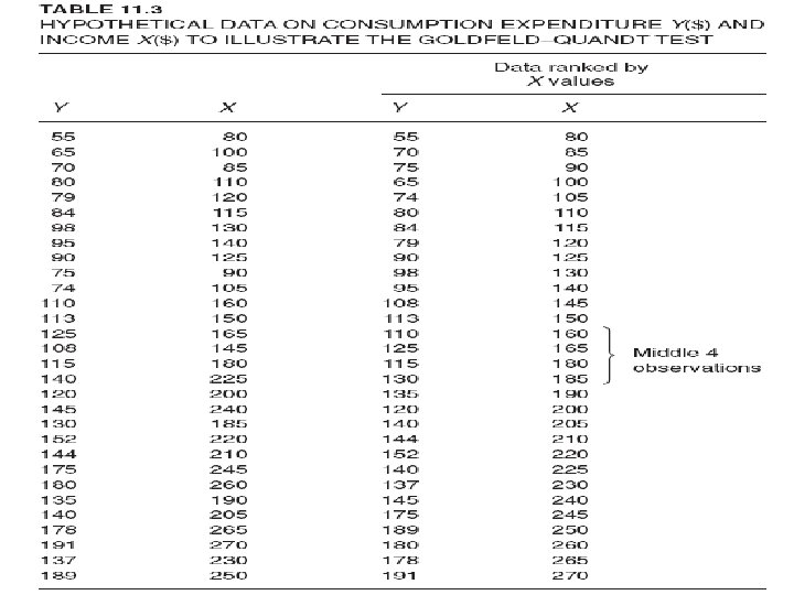
• • To illustrate the Goldfeld–Quandt test, we present in Table 11. 3 data on consumption expenditure in relation to income for a cross section of 30 families. Suppose we postulate that consumption expenditure is linearly related to income but that heteroscedasticity is present in the data. We further postulate that the nature of heteroscedasticity is as given in (11. 5. 10). The necessary reordering of the data for the application of the test is also presented in Table 11. 3. Dropping the middle 4 observations, the OLS regressions based on the first 13 and the last 13 observations and their associated residual sums of squares are as shown next (standard errors in the parentheses). Regression based on the first 13 observations: Yˆi = 3. 4094 + 0. 6968 Xi (8. 7049) (0. 0744) r 2 = 0. 8887 RSS 1 = 377. 17 df = 11 Regression based on the last 13 observations: Yˆi = − 28. 0272 + 0. 7941 Xi (30. 6421) (0. 1319) r 2 = 0. 7681 RSS 2 = 1536. 8 df = 11 From these results we obtain λ = (RSS 2/df)/(RSS 1/df) = (1536. 8/11)/(377. 17/11) λ = 4. 07 The critical F value for 11 numerator and 11 denominator df at the 5 percent level is 2. 82. Since the estimated F( = λ) value exceeds the critical value, we may conclude that there is heteroscedasticity in the error variance. However, if the level of significance is fixed at 1 percent, we may not reject the assumption of homoscedasticity. (Why? ) Note that the p value of the observed λ is 0. 014.

• • • • • • Breusch–Pagan–Godfrey Test. 21 The success of the Goldfeld–Quandt test depends not only on the value of c (the number of central observations to be omitted) but also on identifying the correct X variable with which to order the observations. This limitation of this test can be avoided if we consider the Breusch–Pagan–Godfrey (BPG) test. To illustrate this test, consider the k-variable linear regression model Yi = β 1 + β 2 X 2 i + ·· ·+βk. Xki + ui (11. 5. 12) Assume that the error variance σ2 i is described as σ2 i = f (α 1 + α 2 Z 2 i + ·· ·+αm. Zmi) (11. 5. 13) that is, σ2 i is some function of the nonstochastic variables Z’s; some or all of the X’s can serve as Z’s. Specifically, assume that σ2 i = α 1 + α 2 Z 2 i +· · ·+αm. Zmi (11. 5. 14) that is, σ2 i is a linear function of the Z’s. If α 2 = α 3 = · · · = αm = 0, σ2 i = α 1, which is a constant. Therefore, to test whether σ2 i is homoscedastic, one can test the hypothesis that α 2 = α 3 = · · · = αm = 0. This is the basic idea behind the Breusch–Pagan test. The actual test procedure is as follows.

• • • • • • Step 1. Estimate (11. 5. 12) by OLS and obtain the residuals ˆu 1, ˆu 2, . . . , ˆun. Step 2. Obtain ˜σ2 = ˆu 2 i /n. Recall from Chapter 4 that this is the maximum likelihood (ML) estimator of σ2. [Note: The OLS estimator is ˆu 2 i /(n− k). ] Step 3. Construct variables pi defined as pi = ˆu 2 i ˜σ2 which is simply each residual squared divided by ˜σ2. Step 4. Regress pi thus constructed on the Z’s as pi = α 1 + α 2 Z 2 i +· · ·+αm. Zmi + vi (11. 5. 15) where vi is the residual term of this regression. Step 5. Obtain the ESS (explained sum of squares) from (11. 5. 15) and define = 1 2 (ESS) (11. 5. 16) Assuming ui are normally distributed, one can show that if there is homoscedasticity and if the sample size n increases indefinitely, then ∼asy χ2 m − 1 (11. 5. 17)

• • • that is, follows the chi-square distribution with (m − 1) degrees of freedom. (Note: asy means asymptotically. ) Therefore, if in an application the computed (= χ2) exceeds the critical χ2 value at the chosen level of significance, one can reject the hypothesis of homoscedasticity; otherwise one does not reject it. The reader may wonder why BPG chose 12 ESS as the test statistic. The reasoning is slightly involved and is left for the references. 22 EXAMPLE 11. 5

• • • • • White’s General Heteroscedasticity Test. Unlike the Goldfeld– Quandt test, which requires reordering the observations with respect to the X variable that supposedly caused heteroscedasticity, or the BPG test, which is sensitive to the normality assumption, the general test of heteroscedasticity proposed by White does not rely on the normality assumption and is easy to implement. 24 As an illustration of the basic idea, consider the following three-variable regression model (the generalization to the k-variable model is straightforward): Yi = β 1 + β 2 X 2 i + β 3 X 3 i + ui (11. 5. 21) The White test proceeds as follows: Step 1. Given the data, we estimate (11. 5. 21) and obtain the residuals, ˆui. Step 2. We then run the following (auxiliary) regression: ˆu 2 i = α 1 + α 2 X 2 i + α 3 X 3 i + α 4 X 2 2 i + α 5 X 2 3 i + α 6 X 2 i X 3 i + vi (11. 5. 22)2

• • • • • • That is, the squared residuals from the original regression are regressed on the original X variables or regressors, their squared values, and the cross product(s) of the regressors. Higher powers of regressors can also be introduced. Note that there is a constant term in this equation even though the original regression may or may not contain it. Obtain the R 2 from this (auxiliary) regression. Step 3. Under the null hypothesis that there is no heteroscedasticity, it can be shown that sample size (n) times the R 2 obtained from the auxiliary regression asymptotically follows the chi-square distribution with df equal to the number of regressors (excluding the constant term) in the auxiliary regression. That is, n · R 2 ∼asy χ2 df (11. 5. 23) where df is as defined previously. In our example, there are 5 df since there are 5 regressors in the auxiliary regression. Step 4. If the chi-square value obtained in (11. 5. 23) exceeds the critical chi-square value at the chosen level of significance, the conclusion is that there is heteroscedasticity. If it does not exceed the critical chi-square value, there is no heteroscedasticity, which is to say that in the auxiliary regression (11. 5. 21), α 2 = α 3 = α 4 = α 5 = α 6= 0 (see footnote 25). EXAMPLE 11. 6

• A comment is in order regarding the White test. If a model has several • regressors, then introducing all the regressors, their squared (or higherpowered) • terms, and their cross products can quickly consume degrees of • freedom. Therefore, one must use caution in using the test. 28 • In cases where the White test statistic given in (11. 5. 25) is statistically significant, • heteroscedasticity may not necessarily be the cause, but specification • errors, about which more will be said in Chapter 13 (recall point 5 of • Section 11. 1). In other words, the White test can be a test of (pure) heteroscedasticity • or specification error or both. It has been argued that if • no cross-product terms are present in the White test procedure, then it is a • test of pure heteroscedasticity. If cross-product terms are present, then it is • a test of both heteroscedasticity and specification bias. 29

• • • • 11. 6 REMEDIAL MEASURES As we have seen, heteroscedasticity does not destroy the unbiasedness and consistency properties of the OLS estimators, but they are no longer efficient, not even asymptotically (i. e. , large sample size). This lack of efficiency makes the usual hypothesis-testing procedure of dubious value. Therefore, remedial measures may be called for. There are two approaches to remediation: when σ2 i is known and when σ2 i is not known. When σ2 i Is Known: The Method of Weighted Least Squares As we have seen in Section 11. 3, if σ2 i is known, the most straightforward method of correcting heteroscedasticity is by means of weighted least squares, for the estimators thus obtained are BLUE. EXAMPLE 11. 7

• • • • • When σi 2 Is Not Known As noted earlier, if true σ2 i are known, we can use the WLS method to obtain BLUE estimators. Since the true σ2 i are rarely known, is there a way of obtaining consistent (in the statistical sense) estimates of the variances and covariances of OLS estimators even if there is heteroscedasticity? The answer is yes. White’s Heteroscedasticity-Consistent Variances and Standard Errors. White has shown that this estimate can be performed so that asymptotically valid (i. e. , large-sample) statistical inferences can be made about the true parameter values. 32 We will not present the mathematical details, for they are beyond the scope of this book. However, Appendix 11 A. 4 outlines White’s procedure. Nowadays, several computer packages present White’s heteroscedasticity-corrected variances and standard errors along with the usual OLS variances and standard errors. 33 Incidentally, White’s heteroscedasticity-corrected standard errors are also known as robust standard errors. EXAMPLE 11. 8

• • • • As the preceding results show, (White’s) heteroscedasticity-corrected standard errors are considerably larger than the OLS standard errors and therefore the estimated t values are much smaller than those obtained by OLS. On the basis of the latter, both the regressors are statistically significant at the 5 percent level, whereas on the basis of White estimators they are not. However, it should be pointed out that White’s heteroscedasticity-corrected standard errors can be larger or smaller than the uncorrected standard errors. Since White’s heteroscedasticity-consistent estimators of the variances are now available in established regression packages, it is recommended that the reader report them. As Wallace and Silver note: Generally speaking, it is probably a good idea to use the WHITE option [available in regression programs] routinely, perhaps comparing the output with regular OLS output as a check to see whether heteroscedasticity is a serious problem in a particular set of data. 3

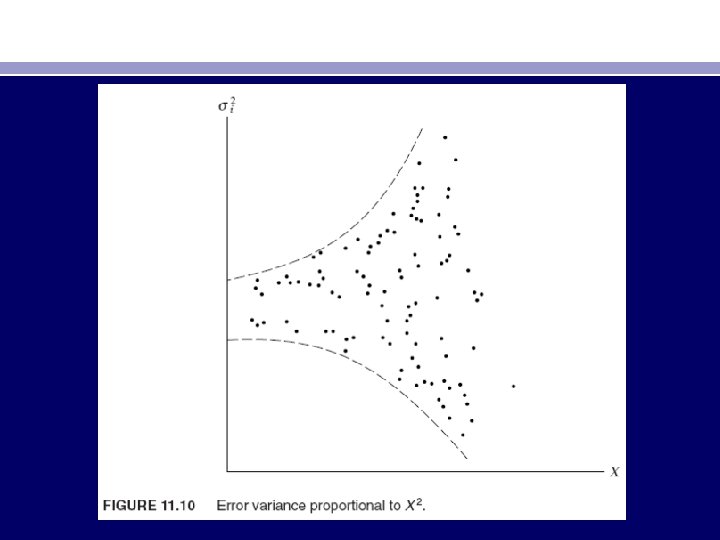
• • • • • • • • • • Plausible Assumptions about Heteroscedasticity Pattern. Apart from being a large-sample procedure, one drawback of the White procedure is that the estimators thus obtained may not be so efficient as those obtained by methods that transform data to reflect specific types of heteroscedasticity. To illustrate this, let us revert to the two-variable regression model: Yi = β 1 + β 2 Xi + ui We now consider several assumptions about the pattern of heteroscedasticity. Assumption 1: The error variance is proportional to X 2 i: E u 2 i = σ2 X 2 i (11. 6. 5)36 If, as a matter of “speculation, ” graphical methods, or Park and Glejser approaches, it is believed that the variance of ui is proportional to the square of the explanatory variable X (see Figure 11. 10), one may transform the original model as follows. Divide the original model through by Xi : Yi Xi = β 1 Xi + β 2 + ui Xi = β 1 1 Xi + β 2 + vi (11. 6. 6) where vi is the transformed disturbance term, equal to ui/Xi. Now it is easy to verify that Ev 2 i = Eui Xi 2 = 1 X 2 i Eu 2 i = σ2 using (11. 6. 5)

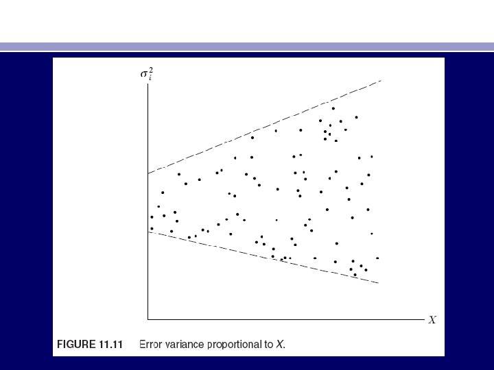
• • • • • • Hence the variance of vi is now homoscedastic, and one may proceed to apply OLS to the transformed equation (11. 6. 6), regressing Yi/Xi on 1/Xi. Notice that in the transformed regression the intercept term β 2 is the slope coefficient in the original equation and the slope coefficient β 1 is the intercept term in the original model. Therefore, to get back to the original model we shall have to multiply the estimated (11. 6. 6) by Xi. An application of this transformation is given in exercise 11. 20. Assumption 2: The error variance is proportional to Xi. The square root transformation: Eu 2 i = σ2 Xi (11. 6. 7) If it is believed that the variance of ui, instead of being proportional to the squared Xi, is proportional to Xi itself, then the original model can be transformed as follows (see Figure 11. 11): Yi √Xi = β 1 √Xi + β 2 Xi + ui √Xi = β 1 1 √Xi + β 2 Xi + vi (11. 6. 8) where vi = ui/√Xi and where Xi > 0.

• • • • • • • Given assumption 2, one can readily verify that E(v 2 i ) = σ2, a homoscedastic situation. Therefore, one may proceed to apply OLS to (11. 6. 8), regressing Yi/√Xi on 1/√Xi and √Xi. Note an important feature of the transformed model: It has no intercept term. Therefore, one will have to use the regression-through-the-origin model to estimate β 1 and β 2. Having run (11. 6. 8), one can get back to the original model simply by multiplying (11. 6. 8) by √Xi. Assumption 3: The error variance is proportional to the square of the mean value of Y. Eu 2 i = σ2[E(Yi )]2 (11. 6. 9) Equation (11. 6. 9) postulates that the variance of ui is proportional to the square of the expected value of Y (see Figure 11. 8 e). Now E(Yi) = β 1 + β 2 Xi Therefore, if we transform the original equation as follows, Yi E(Yi) = β 1 E(Yi) + β 2 Xi E(Yi) + ui E(Yi) = β 1 1 E(Yi) + β 2 Xi E(Yi) + vi (11. 6. 10)

• • • • • • where vi = ui/E(Yi), it can be seen that E(v 2 i ) = σ2; that is, the disturbances vi are homoscedastic. Hence, it is regression (11. 6. 10) that will satisfy the homoscedasticity assumption of the classical linear regression model. The transformation (11. 6. 10) is, however, inoperational because E(Yi) depends on β 1 and β 2, which are unknown. Of course, we know Yˆi = βˆ1 + βˆ2 Xi , which is an estimator of E(Yi). Therefore, we may proceed in two steps: First, we run the usual OLS regression, disregarding the heteroscedasticity problem, and obtain Yˆi. Then, using the estimated Yˆi, we transform our model as follows: Yi Yˆi = β 1 1 Yˆi + β 2 Xi Yˆi + vi (11. 6. 11) where vi = (ui/Yˆi). In Step 2, we run the regression (11. 6. 11). Although Yˆi are not exactly E(Yi), they are consistent estimators; that is, as the sample size increases indefinitely, they converge to true E(Yi). Hence, the transformation (11. 6. 11) will perform satisfactorily in practice if the sample size is reasonably large. Assumption 4: A log transformation such as ln. Yi = β 1 + β 2 ln Xi + ui (11. 6. 12) very often reduces heteroscedasticity when compared with the regression Yi = β 1 + β 2 Xi + ui

• • • • • This result arises because log transformation compresses the scales in which the variables are measured, thereby reducing a tenfold difference between two values to a twofold difference. Thus, the number 80 is 10 times the number 8, but ln 80 (= 4. 3280) is about twice as large as ln 8 (= 2. 0794). An additional advantage of the log transformation is that the slope coefficient β 2 measures the elasticity of Y with respect to X, that is, the percentage change in Y for a percentage change in X. For example, if Y is consumption and X is income, β 2 in (11. 6. 12) will measure income elasticity, whereas in the original model β 2 measures only the rate of change of mean consumption for a unit change in income. It is one reason why the log models are quite popular in empirical econometrics. (For some of the problems associated with log transformation, see exercise 11. 4. ) To conclude our discussion of the remedial measures, we reemphasize that all the transformations discussed previously are ad hoc; we are essentially speculating about the nature of σ2 i. Which of the transformations discussed previously will work will depend on the nature of the problem and the severity of heteroscedasticity. There are some additional problems with the transformations we have considered that should be borne

• • • • • in mind: 1. When we go beyond the two-variable model, we may not know a priori which of the X variables should be chosen for transforming the data. 37 2. Log transformation as discussed in Assumption 4 is not applicable if some of the Y and X values are zero or negative. 38 3. Then there is the problem of spurious correlation. This term, due to Karl Pearson, refers to the situation where correlation is found to be present between the ratios of variables even though the original variables are uncorrelated or random. 39 Thus, in the model Yi = β 1+ β 2 Xi + ui , Y and X may not be correlated but in the transformed model Yi/Xi = β 1(1/Xi) + β 2, Yi/Xi and 1/Xi are often found to be correlated. 4. When σ2 i are not directly known and are estimated from one or more of the transformations that we have discussed earlier, all our testing procedures using the t tests, F tests, etc. , are strictly speaking valid only in large samples. Therefore, one has to be careful in interpreting the results based on the various transformations in small or finite samples. 40

• What happens to OLS estimators and their variances if we introduce heteroscedasticity by letting E(u 2 i ) = σ2 i but retain all other assumptions of the classical model? Let us revert to the two-variable model: • Y i = β 1 + β 2 X i + ui • Applying the usual formula, the OLS estimator of β 2 is • but its variance is now given by the following expression:

• which is obviously different from the usual variance formula obtained under the assumption of homoscedasticity, namely, • Of course, if σ2 i = σ2 for each i, the two formulas will be identical. Recall that βˆ2 is best linear unbiased estimator (BLUE) if the assumptions of the classical model, including homoscedasticity, hold. Is it still BLUE when we drop only the homoscedasticity assumption and replace it with the assumption of heteroscedasticity? It is easy to prove that βˆ2 is still linear and unbiased. As a matter of fact, as shown in Appendix 3 A, Section 3 A. 2, to establish the unbiasedness of βˆ2 it is not necessary that the disturbances (ui) be homoscedastic. In fact, the variance of ui , homoscedastic or heteroscedastic, plays no part in the determination of the unbiasedness property. Recall that in Appendix 3 A, Section 3 A. 7, we showed that βˆ2 is a consistent estimator under the assumptions of the classical linear regression model. Although we will not prove it, it can be shown that βˆ2 is a consistent estimator despite heteroscedasticity; that is, as the sample size increases indefinitely, the estimated β 2 converges to its true value. Furthermore, it can also be shown that under certain conditions (called regularity conditions), βˆ2 is asymptotically normally distributed. Of course, what we have said about βˆ2 also holds true of other parameters of a multiple regression model. •

• Granted that βˆ2 is still linear unbiased and consistent, is it “efficient” or “best”; that is, does it have minimum variance in the class of unbiased estimators? And is that minimum variance given by Eq. (11. 2. 2)? The answer is no to both the questions: βˆ2 is no longer best and the minimum variance is not given by (11. 2. 2). Then what is BLUE in the presence of heteroscedasticity? The answer is given in the following section.

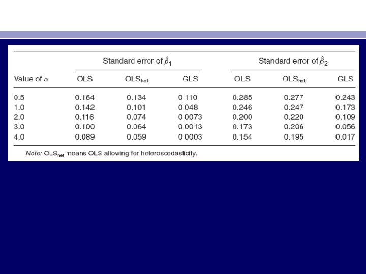
• To throw more light on this topic, we refer to a Monte Carlo study conducted by Davidson and Mac. Kinnon. They consider the following simple model, which in our notation is • Y i = β 1 + β 2 X i + ui (11. 4. 1) • They assume that β 1 = 1, β 2 = 1, and ui ∼ N(0, Xαi ). As the last expression shows, they assume that the error variance is heteroscedastic and is related to the value of the regressor X with power α. If, for example, α = 1, the error variance is proportional to the value of X; if α = 2, the error variance is proportional to the square of the value of X, and so on. In Section 11. 6 we will consider the logic behind such a procedure. Based on 20, 000 replications and allowing for various values for α, they obtain the standard errors of the two regression coefficients using OLS [see Eq. (11. 2. 3)], OLS allowing for heteroscedasticity [see Eq. (11. 2. 2)], and GLS [see Eq. (11. 3. 9)]. We quote their results for selected values of α:

• • The most striking feature of these results is that OLS, with or without correction for heteroscedasticity, consistently overestimates the true standard error obtained by the (correct) GLS procedure, especially for large values of α, thus establishing the superiority of GLS. These results also show that if we do not use GLS and rely on OLS—allowing for or not allowing for heteroscedasticity— the picture is mixed. The usual OLS standard errors are either too large (for the intercept) or too small (for the slope coefficient) in relation to those obtained by OLS allowing for heteroscedasticity. The message is clear: In the presence of heteroscedasticity, use GLS. However, for reasons explained later in the chapter, in practice it is not always easy to apply GLS. Also, as we discuss later, unless heteroscedasticity is very severe, one may not abandon OLS in favor of GLS or WLS. From the preceding discussion it is clear that heteroscedasticity is potentially a serious problem and the researcher needs to know whether it is present in a given situation. If its presence is detected, then one can take corrective action, such as using the weighted least-squares regression or some other technique. Before we turn to examining the various corrective procedures, however, we must first find out whether heteroscedasticity is present or likely to be present in a given case. This topic is discussed in the following section.

• A Technical Note • Although we have stated that, in cases of heteroscedasticity, it is the GLS, not the OLS, that is BLUE, there are examples where OLS can be BLUE, despite heteroscedasticity. 8 But such examples are infrequent in practice.