Heteroskedasticity Nature and Detection 1 Aims and Learning

Heteroskedasticity: Nature and Detection 1

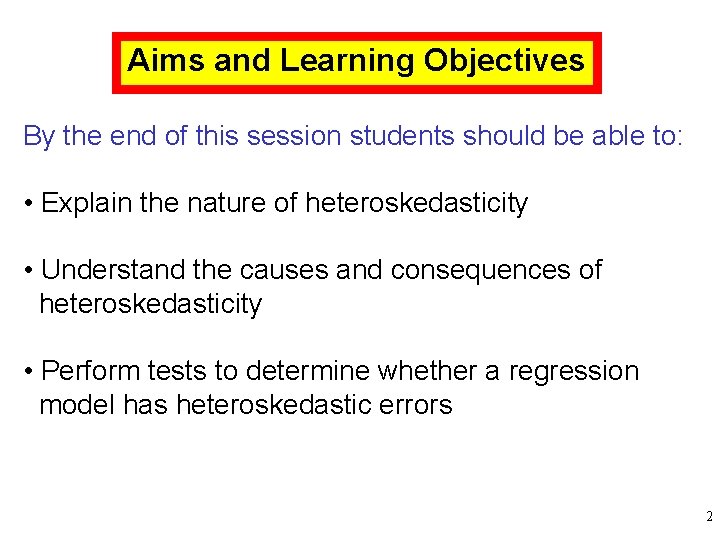
Aims and Learning Objectives By the end of this session students should be able to: • Explain the nature of heteroskedasticity • Understand the causes and consequences of heteroskedasticity • Perform tests to determine whether a regression model has heteroskedastic errors 2

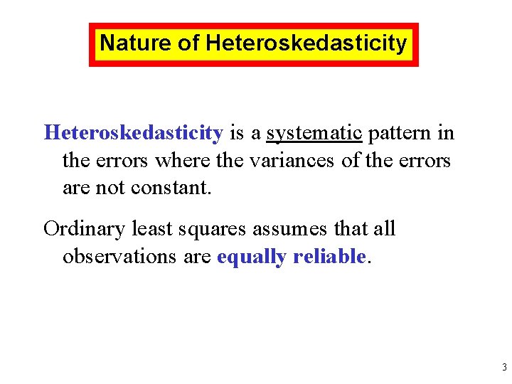
Nature of Heteroskedasticity is a systematic pattern in the errors where the variances of the errors are not constant. Ordinary least squares assumes that all observations are equally reliable. 3

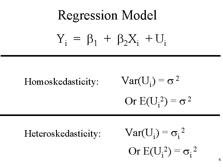
Regression Model Yi = 1 + 2 Xi + Ui Homoskedasticity: Var(Ui) = 2 Or E(Ui 2) = 2 Heteroskedasticity: Var(Ui) = i 2 Or E(Ui 2) = i 2 4

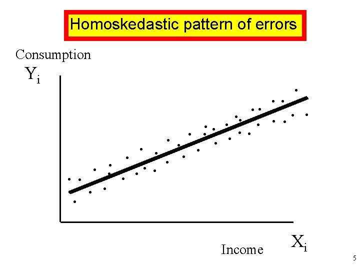
Homoskedastic pattern of errors Consumption Yi . . Income Xi 5

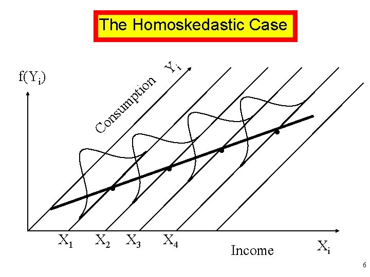
The Homoskedastic Case f(Yi) n o ti Yi p m u s n o C . . X 1 X 2 X 3 X 4 . . Income Xi 6

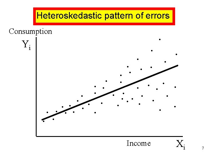
Heteroskedastic pattern of errors Consumption Yi . . . Income Xi 7

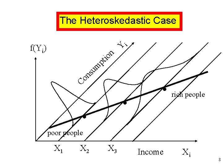
The Heteroskedastic Case i Y f(Yi) n o ti p m u s n o C . . . rich people poor people X 1 X 2 X 3 Income Xi 8

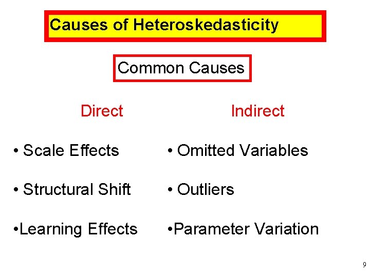
Causes of Heteroskedasticity Common Causes Direct Indirect • Scale Effects • Omitted Variables • Structural Shift • Outliers • Learning Effects • Parameter Variation 9

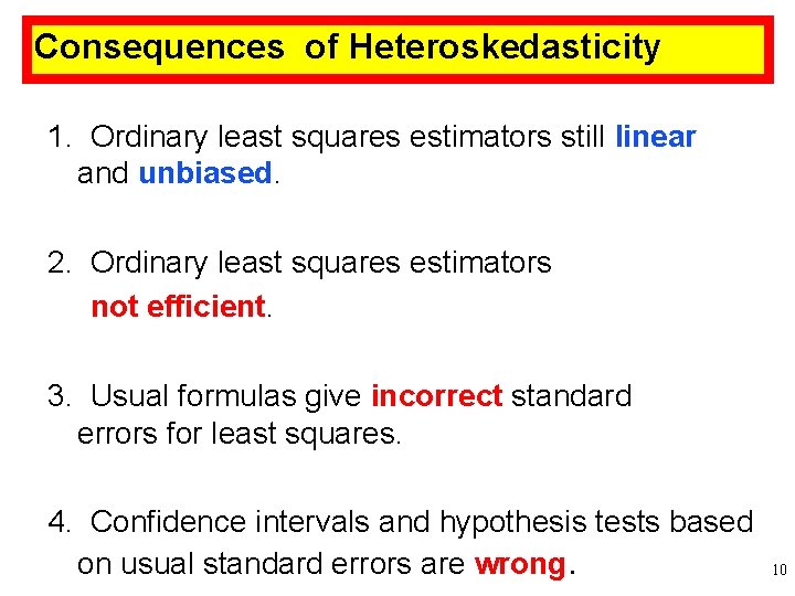
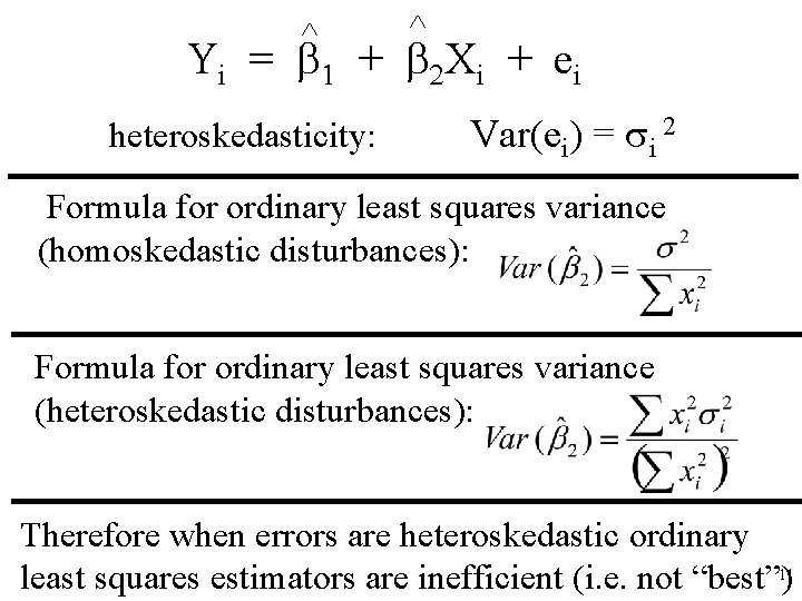
Consequences of Heteroskedasticity 1. Ordinary least squares estimators still linear and unbiased. 2. Ordinary least squares estimators not efficient. 3. Usual formulas give incorrect standard errors for least squares. 4. Confidence intervals and hypothesis tests based on usual standard errors are wrong. 10

^ ^ Yi = 1 + 2 Xi + ei heteroskedasticity: Var(ei) = i 2 Formula for ordinary least squares variance (homoskedastic disturbances): Formula for ordinary least squares variance (heteroskedastic disturbances): Therefore when errors are heteroskedastic ordinary least squares estimators are inefficient (i. e. not “best”)11

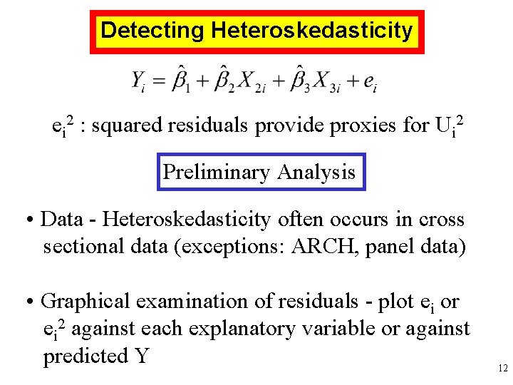
Detecting Heteroskedasticity ei 2 : squared residuals provide proxies for Ui 2 Preliminary Analysis • Data - Heteroskedasticity often occurs in cross sectional data (exceptions: ARCH, panel data) • Graphical examination of residuals - plot ei or ei 2 against each explanatory variable or against predicted Y 12

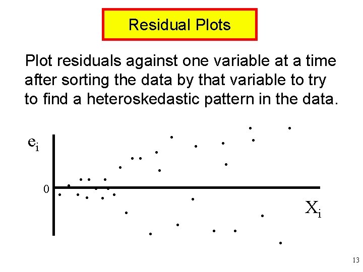
Residual Plots Plot residuals against one variable at a time after sorting the data by that variable to try to find a heteroskedastic pattern in the data. ei 0 . . . . Xi . . 13

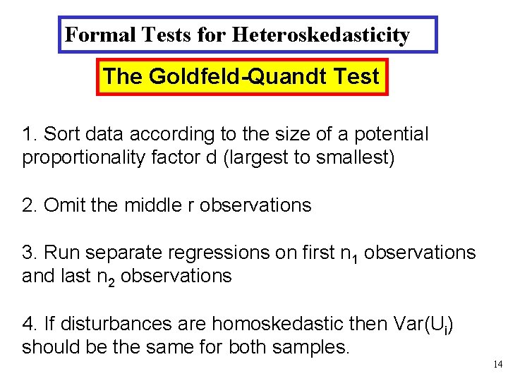
Formal Tests for Heteroskedasticity The Goldfeld-Quandt Test 1. Sort data according to the size of a potential proportionality factor d (largest to smallest) 2. Omit the middle r observations 3. Run separate regressions on first n 1 observations and last n 2 observations 4. If disturbances are homoskedastic then Var(Ui) should be the same for both samples. 14

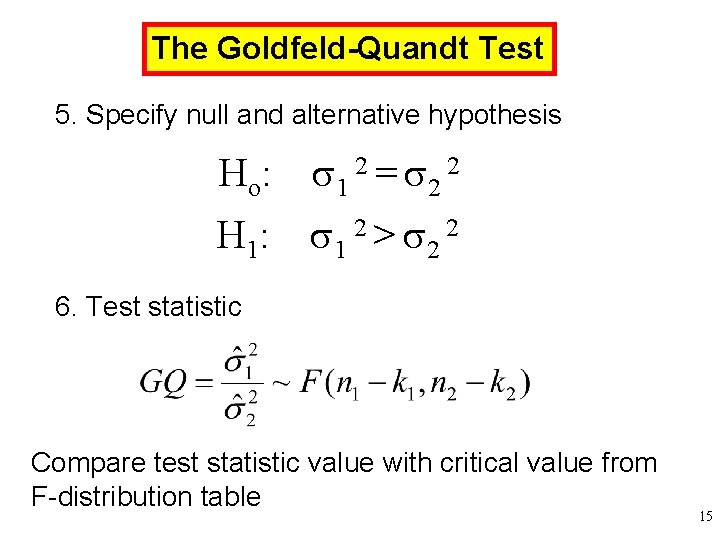
The Goldfeld-Quandt Test 5. Specify null and alternative hypothesis Ho: 1 2 = 2 2 H 1: 1 2 > 2 2 6. Test statistic Compare test statistic value with critical value from F-distribution table 15

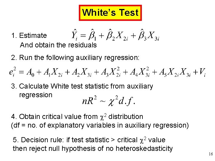
White’s Test 1. Estimate And obtain the residuals 2. Run the following auxiliary regression: 3. Calculate White test statistic from auxiliary regression 4. Obtain critical value from 2 distribution (df = no. of explanatory variables in auxiliary regression) 5. Decision rule: if test statistic > critical 2 value then reject null hypothesis of no heteroskedasticity 16

Summary In this lecture we have: 1. Analysed theoretical causes and consequences of heteroskedasticity 2. Outlined a number of tests which can be used to detect the presence of heteroskedastic errors 17