13 1 The Chisquare GoodnessofFit test Agenda for

13. 1 The Chi-square Goodness-of-Fit test Agenda for 4/8 and 4/9 NEW GROUPS – pick your own CHOOSE Wisely (no less than 3 members) Introduction of X 2 Discussion of Homework

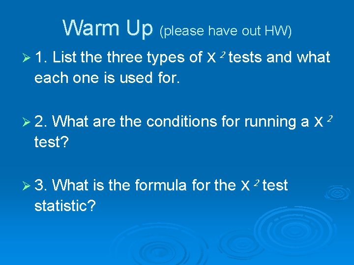
Warm Up (please have out HW) Ø 1. List the three types of X 2 tests and what each one is used for. Ø 2. What are the conditions for running a test? Ø 3. What is the formula for the statistic? X 2 test X 2

X 2 - Chi (Ki) Ø The chi-square test is a statistic used to compare and decide whether two or more populations, variables or characteristics are the same as a claim.

X 2 - Chi (Ki) Ø It does not matter what the distributions of the populations are so long as the relative frequencies are known for each population or the population and some standard population frequencies.

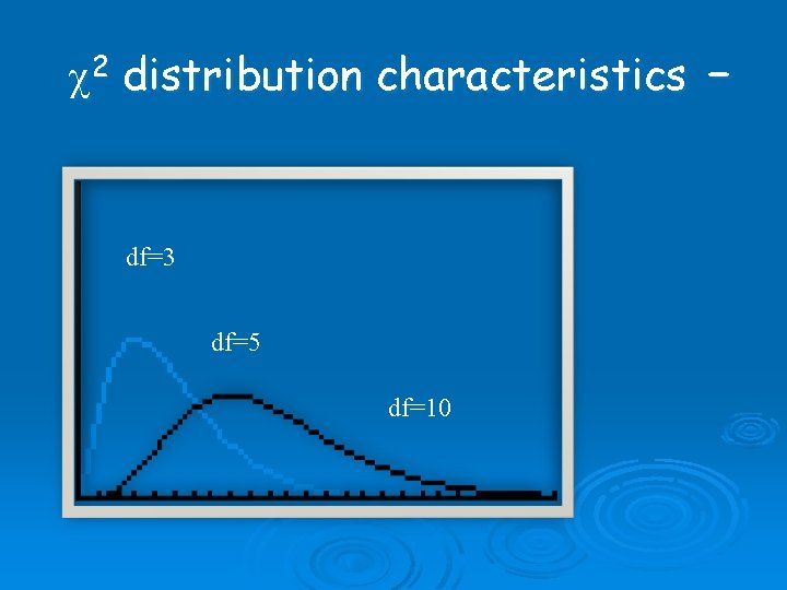
c 2 distribution characteristics – df=3 df=5 df=10

c 2 distribution characteristics Ø Different df have different curves Ø Skewed right Ø As df increases, curve shifts toward right & becomes more like a normal curve

1 st Test - X 2 Goodness of Fit Ø Goodness of fit – used to test to see if the null hypothesis population distribution is the same as a referenced distribution. Ø (ex: is the companies claim actually true? )

nd 2 2 - X Test of Homogeneity Ø Homogeneity – is an overall test that tells us whether the data give a good indication that the categorical variable is the same in multiple populations. Ø (ex: do python eggs hatch more or less in cold, neutral or warm waters? )

rd 3 – X 2 Test of Association/Independence Ø Test for Independence – used to test the association/independence between categorical variables Ø (ex: is there a relationship between patient survival and pet ownership? )

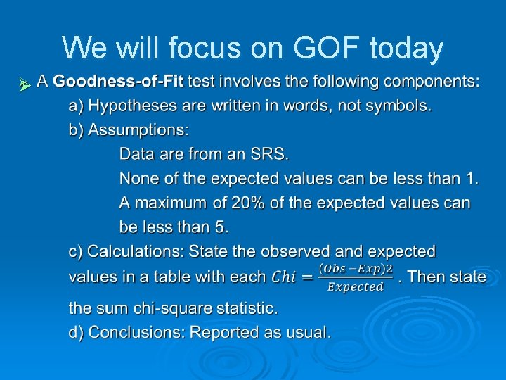
We will focus on GOF today Ø

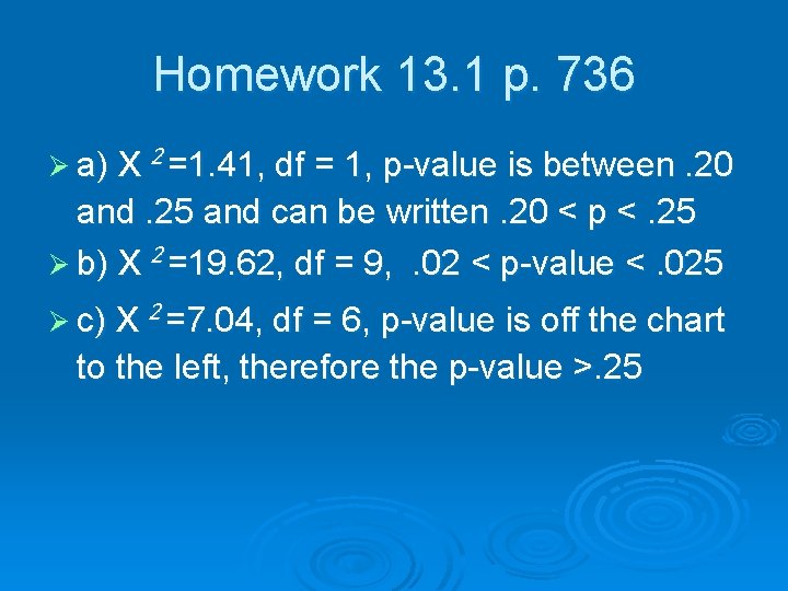
Homework 13. 1 p. 736 Ø a) X 2 =1. 41, df = 1, p-value is between. 20 and. 25 and can be written. 20 < p <. 25 Ø b) X 2 =19. 62, df = 9, . 02 < p-value <. 025 Ø c) X 2 =7. 04, df = 6, p-value is off the chart to the left, therefore the p-value >. 25

k r o w e m o H 2. 3 #1 u o y e Ar ? d e i r r a m 6 3 7 e Pag

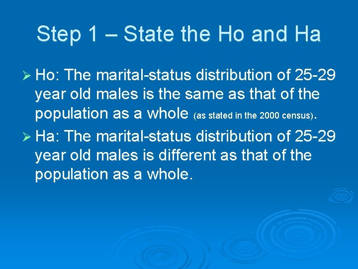
Step 1 – State the Ho and Ha Ø Ho: The marital-status distribution of 25 -29 year old males is the same as that of the population as a whole (as stated in the 2000 census). Ø Ha: The marital-status distribution of 25 -29 year old males is different as that of the population as a whole.

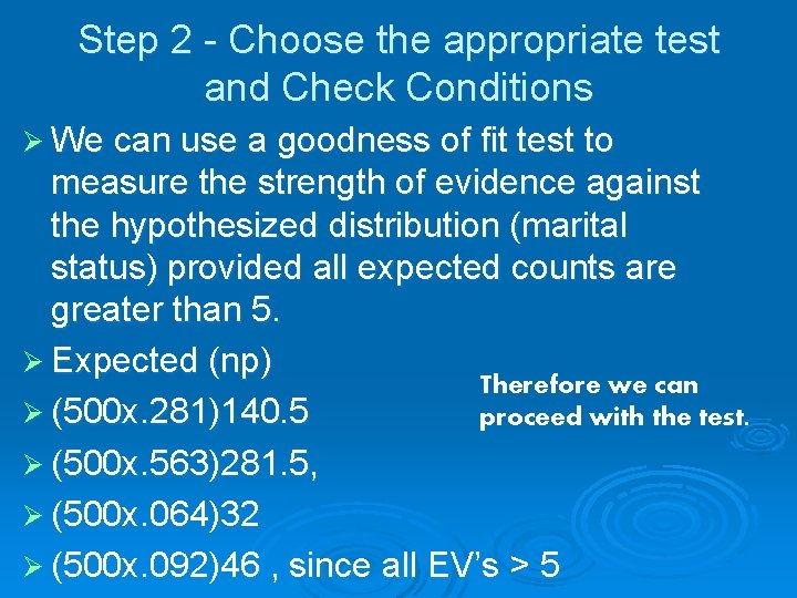
Step 2 - Choose the appropriate test and Check Conditions Ø We can use a goodness of fit test to measure the strength of evidence against the hypothesized distribution (marital status) provided all expected counts are greater than 5. Ø Expected (np) Therefore we can Ø (500 x. 281)140. 5 proceed with the test. Ø (500 x. 563)281. 5, Ø (500 x. 064)32 Ø (500 x. 092)46 , since all EV’s > 5

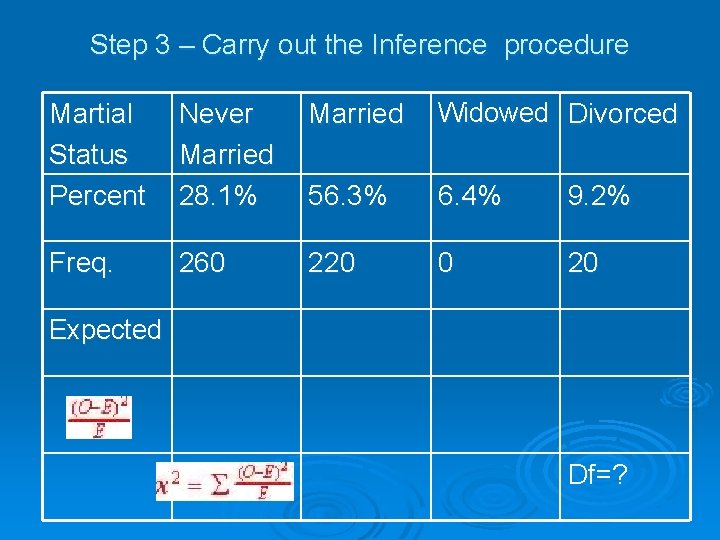
Step 3 – Carry out the Inference procedure Martial Status Percent Never Married 28. 1% Married Widowed Divorced 56. 3% 6. 4% 9. 2% Freq. 260 220 0 20 Expected Df=?

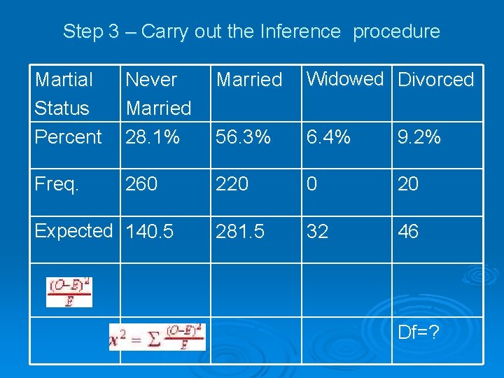
Step 3 – Carry out the Inference procedure Martial Status Percent Never Married 28. 1% Married Widowed Divorced 56. 3% 6. 4% 9. 2% Freq. 260 220 0 20 281. 5 32 46 Expected 140. 5 Df=?

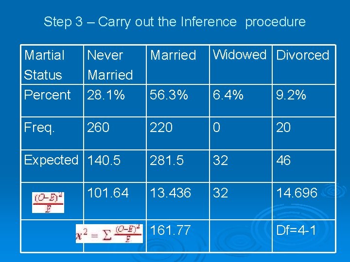
Step 3 – Carry out the Inference procedure Martial Status Percent Never Married 28. 1% Married Widowed Divorced 56. 3% 6. 4% 9. 2% Freq. 260 220 0 20 281. 5 32 46 13. 436 32 14. 696 Expected 140. 5 101. 64 161. 77 Df=4 -1

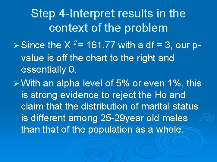
Step 4 -Interpret results in the context of the problem Ø Since the X 2 = 161. 77 with a df = 3, our p- value is off the chart to the right and essentially 0. Ø With an alpha level of 5% or even 1%, this is strong evidence to reject the Ho and claim that the distribution of marital status is different among 25 -29 year old males than that of the population as a whole.

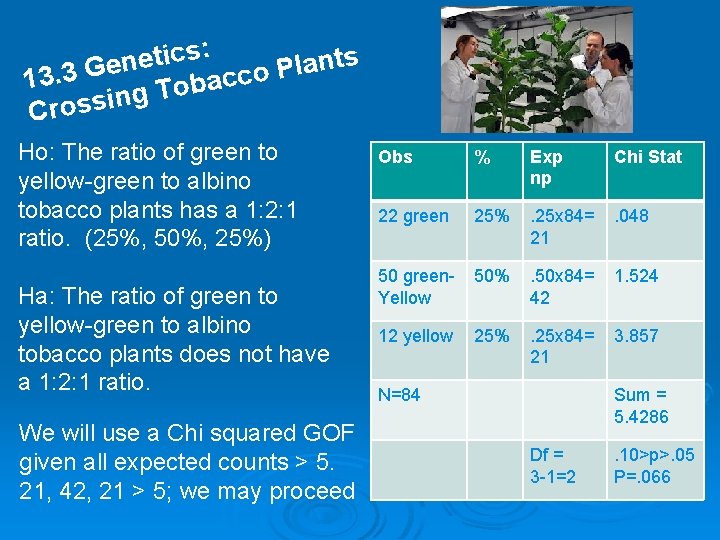
s: c i t ts e n n a e l G P o c c 13. 3 a b To g n i s Cros Ho: The ratio of green to yellow-green to albino tobacco plants has a 1: 2: 1 ratio. (25%, 50%, 25%) Ha: The ratio of green to yellow-green to albino tobacco plants does not have a 1: 2: 1 ratio. We will use a Chi squared GOF given all expected counts > 5. 21, 42, 21 > 5; we may proceed Obs % Exp np Chi Stat 22 green 25% . 25 x 84= 21 . 048 50 green. Yellow 50% . 50 x 84= 42 1. 524 12 yellow 25% . 25 x 84= 21 3. 857 N=84 Sum = 5. 4286 Df = 3 -1=2 . 10>p>. 05 P=. 066

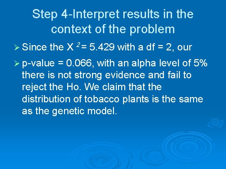
Step 4 -Interpret results in the context of the problem Ø Since the X 2 = 5. 429 with a df = 2, our Ø p-value = 0. 066, with an alpha level of 5% there is not strong evidence and fail to reject the Ho. We claim that the distribution of tobacco plants is the same as the genetic model.

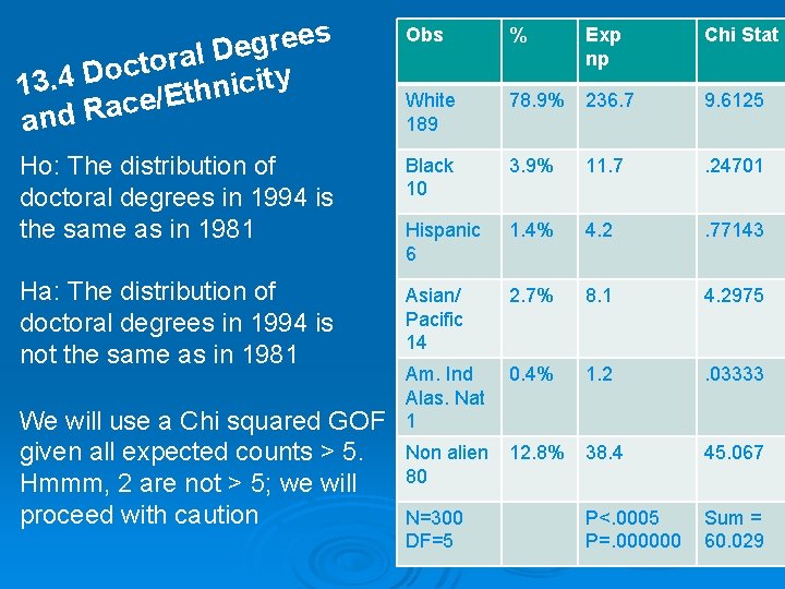
s e e r g e D l a r o ct o D 4. ity c i 13 n h t /E e c a R and Obs % Exp np Chi Stat White 189 78. 9% 236. 7 9. 6125 Ho: The distribution of doctoral degrees in 1994 is the same as in 1981 Black 10 3. 9% 11. 7 . 24701 Hispanic 6 1. 4% 4. 2 . 77143 Ha: The distribution of doctoral degrees in 1994 is not the same as in 1981 Asian/ Pacific 14 2. 7% 8. 1 4. 2975 0. 4% 1. 2 . 03333 We will use a Chi squared GOF given all expected counts > 5. Hmmm, 2 are not > 5; we will proceed with caution Am. Ind Alas. Nat 1 Non alien 80 12. 8% 38. 4 45. 067 P<. 0005 P=. 000000 Sum = 60. 029 N=300 DF=5

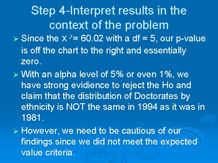
Step 4 -Interpret results in the context of the problem Ø Since the X 2 = 60. 02 with a df = 5, our p-value is off the chart to the right and essentially zero. Ø With an alpha level of 5% or even 1%, we have strong evidience to reject the Ho and claim that the distribution of Doctorates by ethnicity is NOT the same in 1994 as it was in 1981. Ø However, we need to be cautious of our findings since we did not meet the expected value criteria.

Homework Ø Read and take notes 13. 2 Ø Figure out what type of M&M your group wants to bring or you all can choose skittles. You will need to buy ONE LARGE Family Size Bag of the item. Ø Do #’s 13 (13. 1), 14, 16, 20, 22

# 7 - Is your random number generator working? Turn to page 742. We will work a and b as a class.

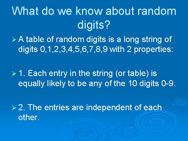
What do we know about random digits? Ø A table of random digits is a long string of digits 0, 1, 2, 3, 4, 5, 6, 7, 8, 9 with 2 properties: Ø 1. Each entry in the string (or table) is equally likely to be any of the 10 digits 0 -9. Ø 2. The entries are independent of each other.

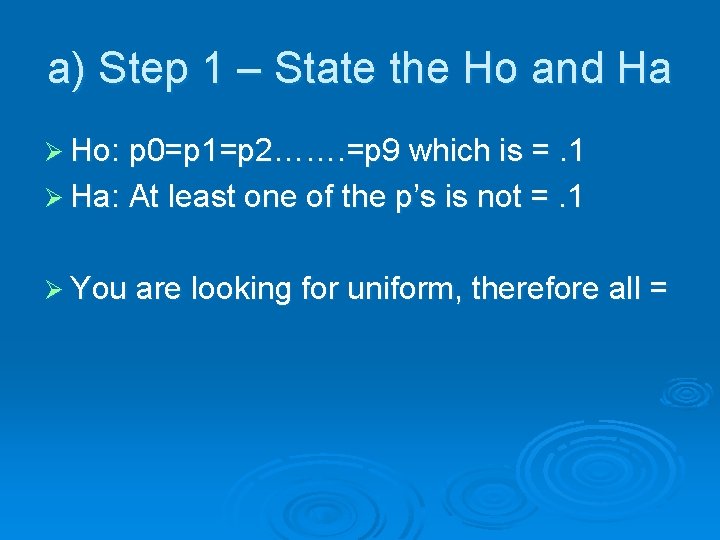
a) Step 1 – State the Ho and Ha Ø Ho: p 0=p 1=p 2……. =p 9 which is =. 1 Ø Ha: At least one of the p’s is not =. 1 Ø You are looking for uniform, therefore all =

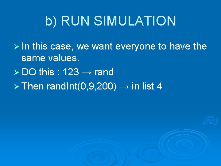
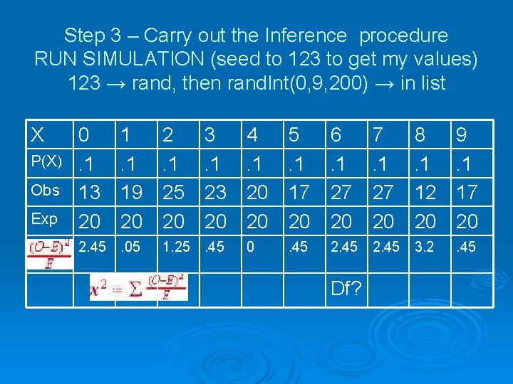
b) RUN SIMULATION Ø In this case, we want everyone to have the same values. Ø DO this : 123 → rand Ø Then rand. Int(0, 9, 200) → in list 4

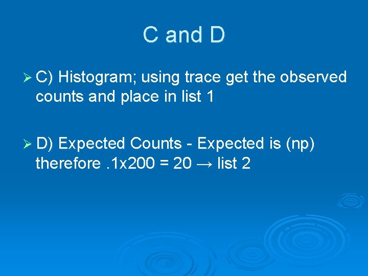
C and D Ø C) Histogram; using trace get the observed counts and place in list 1 Ø D) Expected Counts - Expected is (np) therefore. 1 x 200 = 20 → list 2

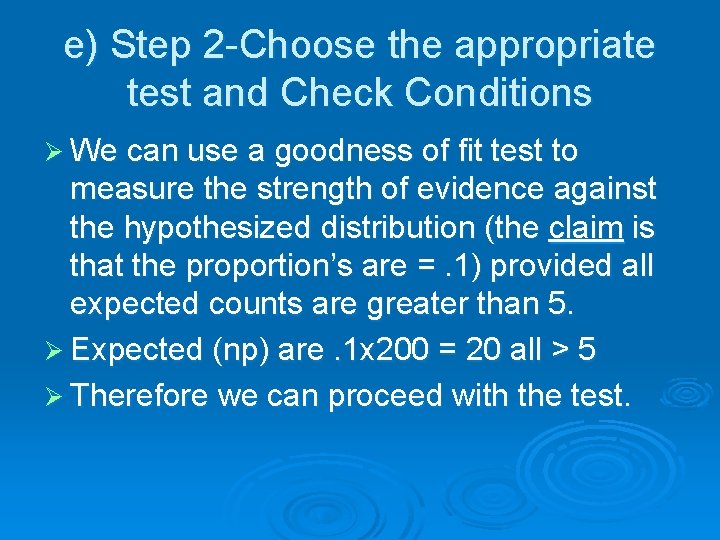
e) Step 2 -Choose the appropriate test and Check Conditions Ø We can use a goodness of fit test to measure the strength of evidence against the hypothesized distribution (the claim is that the proportion’s are =. 1) provided all expected counts are greater than 5. Ø Expected (np) are. 1 x 200 = 20 all > 5 Ø Therefore we can proceed with the test.

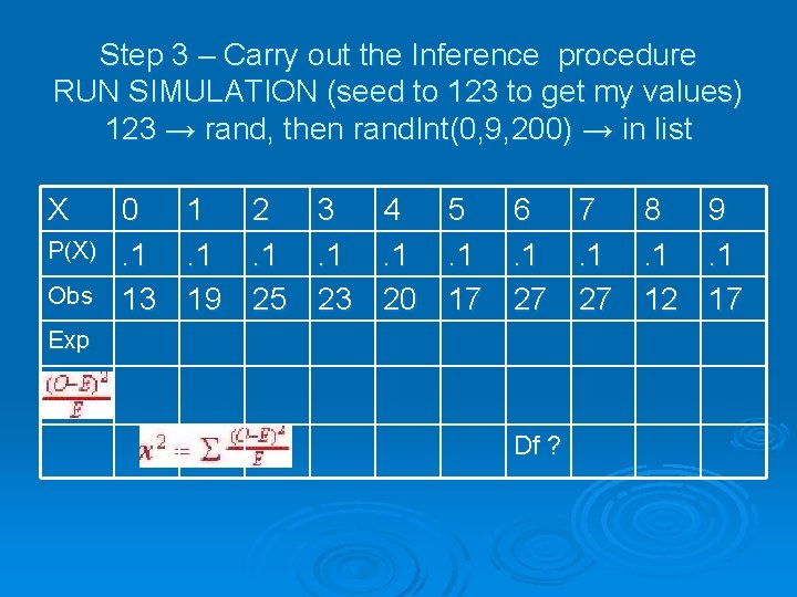
Step 3 – Carry out the Inference procedure RUN SIMULATION (seed to 123 to get my values) 123 → rand, then rand. Int(0, 9, 200) → in list X P(X) 0. 1 1. 1 2. 1 3. 1 4. 1 5. 1 6. 1 Obs Exp Df ? 7. 1 8. 1 9. 1

Step 3 – Carry out the Inference procedure RUN SIMULATION (seed to 123 to get my values) 123 → rand, then rand. Int(0, 9, 200) → in list X P(X) Obs 0. 1 13 1. 1 19 2. 1 25 3. 1 23 4. 1 20 5. 1 17 6. 1 27 Exp Df ? 7. 1 27 8. 1 12 9. 1 17

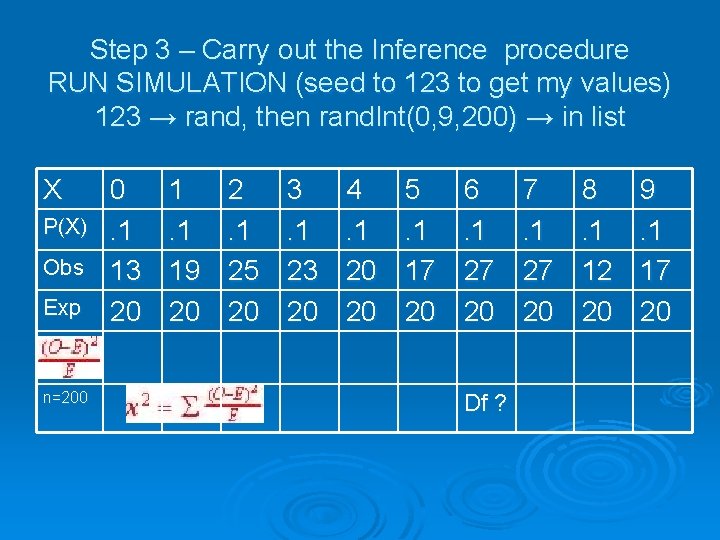
Step 3 – Carry out the Inference procedure RUN SIMULATION (seed to 123 to get my values) 123 → rand, then rand. Int(0, 9, 200) → in list X P(X) Obs Exp n=200 0. 1 13 20 1. 1 19 20 2. 1 25 20 3. 1 23 20 4. 1 20 20 5. 1 17 20 6. 1 27 20 Df ? 7. 1 27 20 8. 1 12 20 9. 1 17 20

Step 3 – Carry out the Inference procedure RUN SIMULATION (seed to 123 to get my values) 123 → rand, then rand. Int(0, 9, 200) → in list X P(X) Obs Exp 0. 1 13 20 1. 1 19 20 2. 45. 05 2. 1 25 20 3. 1 23 20 1. 25. 45 4. 1 20 20 5. 1 17 20 6. 1 27 20 8. 1 12 20 9. 1 17 20 0 . 45 2. 45 3. 2 . 45 Df? 7. 1 27 20

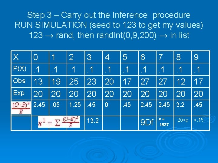
Step 3 – Carry out the Inference procedure RUN SIMULATION (seed to 123 to get my values) 123 → rand, then rand. Int(0, 9, 200) → in list X P(X) Obs Exp 0. 1 13 20 1. 1 19 20 2. 45. 05 2. 1 25 20 3. 1 23 20 1. 25. 45 13. 2 4. 1 20 20 5. 1 17 20 6. 1 27 20 8. 1 12 20 9. 1 17 20 0 . 45 2. 45 3. 2 . 45 P=. 1537 <. 15 9 Df 7. 1 27 20 . 20<p

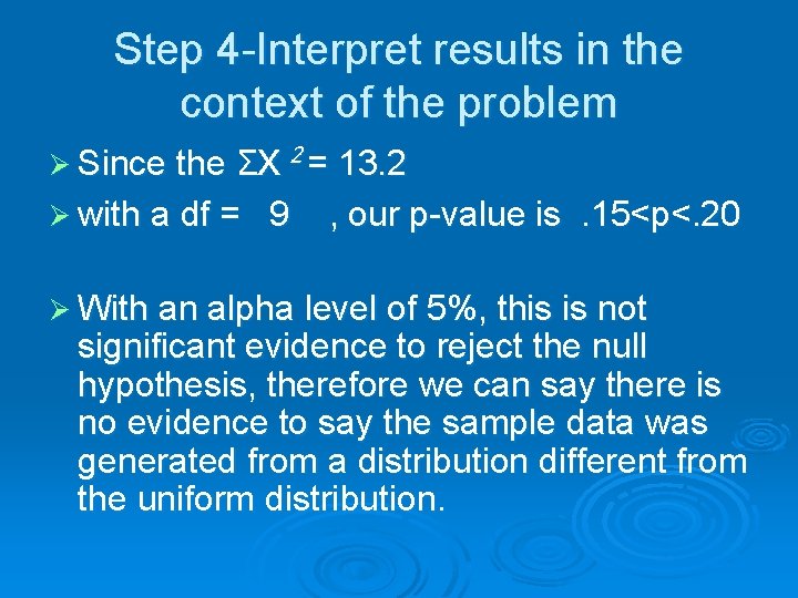
Step 4 -Interpret results in the context of the problem Ø Since the ΣX 2 = 13. 2 Ø with a df = 9 , our p-value is. 15<p<. 20 Ø With an alpha level of 5%, this is not significant evidence to reject the null hypothesis, therefore we can say there is no evidence to say the sample data was generated from a distribution different from the uniform distribution.

Warm Up

Carnival Games # 13 page 744

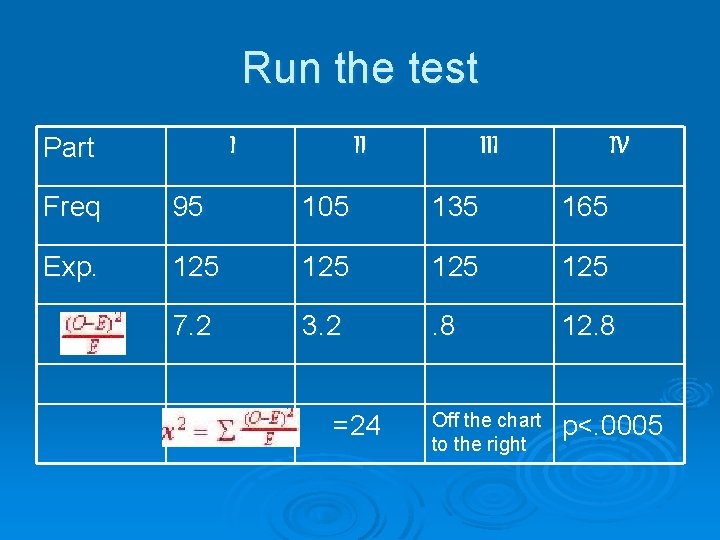
Run the test Part I II IV Freq 95 105 135 165 Exp. 125 125 7. 2 3. 2 . 8 12. 8 Off the chart to the right p<. 0005 =24

What were we thinking? Ho: The carnival wheel is balance and all 4 parts are evenly distributed. Ø Ha: The carnival wheel is not balanced and all 4 parts are NOT evenly distributed. Ø Since all exptected values are > than 5 (E=125) we can use the X 2 test. Ø Running the test gave us a X 2 of 24 w/ 3 df and a p<. 0005 Ø We have sufficient evidence to reject the null and make a claim that the wheel is not balanced. Ø Where is the most significant X 2 ? Ø

2 nd - X 2 Test of Homogeneity (or two way tables) Homogeneity – is an overall test that tells us whether the data give a good indication that the categorical variable is the same in multiple populations. Ø We are testing population proportions for a categorical variable. Ø The null hypothesis states that all the proportions are equal. Ø The alternative states that they are not all equal Ø

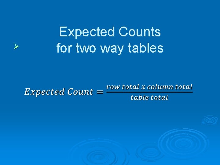
Ø Expected Counts for two way tables

rd 3 – X 2 Test of Association/Independence Test for Independence – used to test the association/independence between categorical variables. Ø An SRS is drawn from a population and observations are classified according to two categorical variables. Ø The null hypothesis is there is NO relationship between the row variable and the column variable. Ø The alternative would state that there is a relationship. Ø

Ø Expected Counts for two way tables

Homework Ø Pulling together 13 Do #25, 39

How to qu it sm oking # 14, 16

Smoking by Students and Their Parents Ø # 20, 22