Visual Grouping and Recognition Jitendra Malik U C

Visual Grouping and Recognition Jitendra Malik U. C. Berkeley

Collaborators • Grouping: Jianbo Shi (CMU), Serge Belongie (UCSD) , Thomas Leung (Fuji) • Database of human segmented images and ecological statistics: David Martin, Charless Fowlkes, Xiaofeng Ren • Recognition: Serge Belongie, Jan Puzicha

The visual system performs • Inference of lightness, shape and spatial relations • Perceptual Organization • Active interaction with environment

A brief history of vision science • 1850 -1900 – Trichromacy, stereopsis, eye movements, contrast, visual acuity. . • 1900 -1950 – Apparent movement, grouping, figure-ground. . • 1950 -2000 – Ecological optics, geometrical analysis of shape cues, physiology of V 1 and extra-striate areas. .

Physiological Optics 1840 -1894

The Empiricist-Nativist debate

The debate. . (and sometimes both were right !) • Helmholtz argued that perception is unconscious inference. Associations are earned through experience. • Hering proposed physiological mechanisms —opponent color channels, contrast mechanisms, conjunctive and disjunctive eye movements. .

The Twentieth Century. . • The Gestalt movement emphasized perceptual organization. – Grouping – Figure/ground – Configuration effects on perception of brightness and lightness

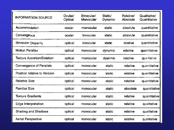
Gibson’s ecological optics (1950) • Emphasized richness of information about shape and surface layout available to a moving observer – Optical flow – Texture Gradients – ( and the classical cues such as stereopsis etc)

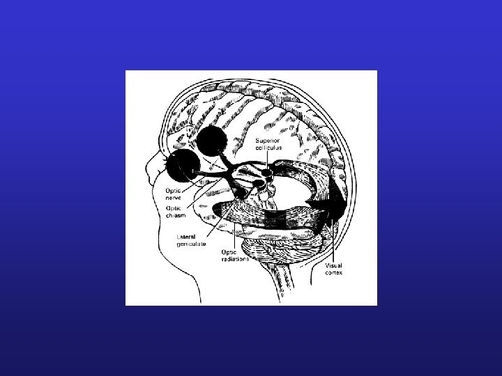
Visual Processing Areas

The visual system performs • Inference of lightness, shape and spatial relations • Perceptual Organization • Active interaction with environment

From Images to Objects

What enables us to parse a scene? – Low level cues • Color/texture • Contours • Motion – Mid level cues • T-junctions • Convexity – High level Cues • Familiar Object • Familiar Motion

Grouping factors

Grouping Factors

The Figure-Ground Problem

Focus of this talk • Provide a mathematical foundation for the grouping problem in terms of the ecological statistics of natural images. – This research agenda was first proposed by Egon Brunswik, more than 50 years ago, who sought to justify Gestalt grouping factors in probabilistic terms.

Outline of talk • Creating a dataset of human segmented images • Measuring ecological statistics of various Gestalt grouping factors • Using these measurements to calibrate and validate approaches to grouping

Outline of talk • Creating a dataset of human segmented images • Measuring ecological statistics of various Gestalt grouping factors • Using these measurements to calibrate and validate approaches to grouping

What kind of segmentations? • What is a valid segmentation? • Is there a correct segmentation? • What granularity?

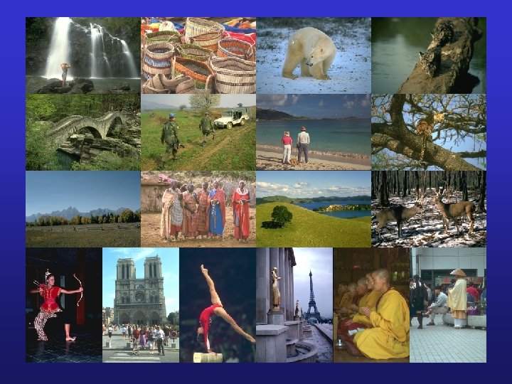
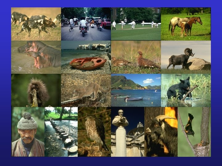
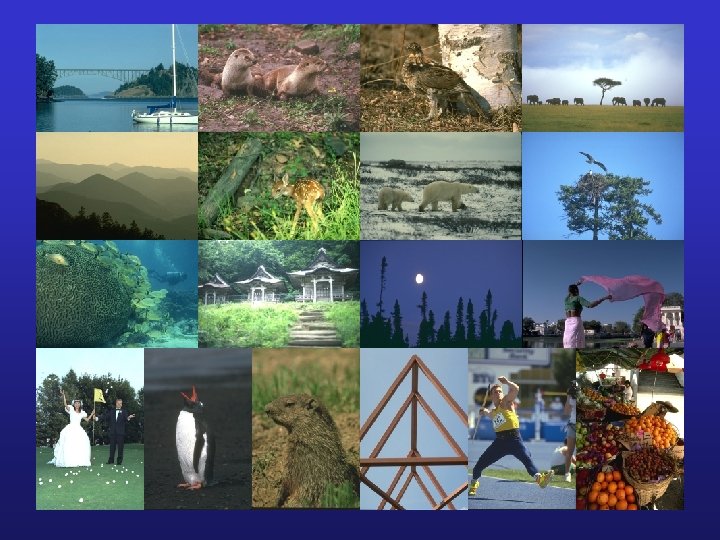
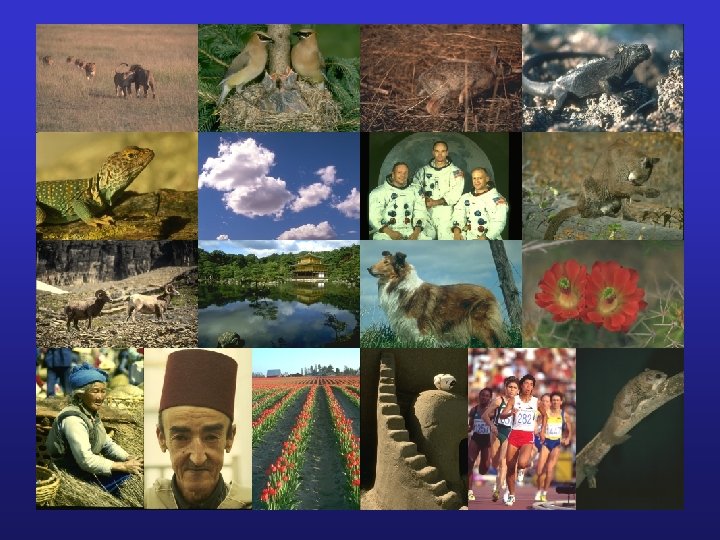
The Image Dataset • 1000 Corel images – Photographs of natural scenes – Texture is common – Large variety of subject matter – 481 x 321 x 24 b

Establishing Ground truth • Def: Segmentation = Partition of image pixels into exclusive sets • Custom tool to facilitate manual segmentation – Java application, on website • Multiple segmentations/image • Currently: 1000 images, 5000 segmentations, 20 subjects – Data collection ongoing • Naïve subjects (UCB undergrads) given simple, non-technical instructions

Directions to Image Segmentors • You will be presented a photographic image • Divide the image into some number of segments, where the segments represent “things” or “parts of things” in the scene • The number of segments is up to you, as it depends on the image. Something between 2 and 30 is likely to be appropriate. • It is important that all of the segments have approximately equal importance.

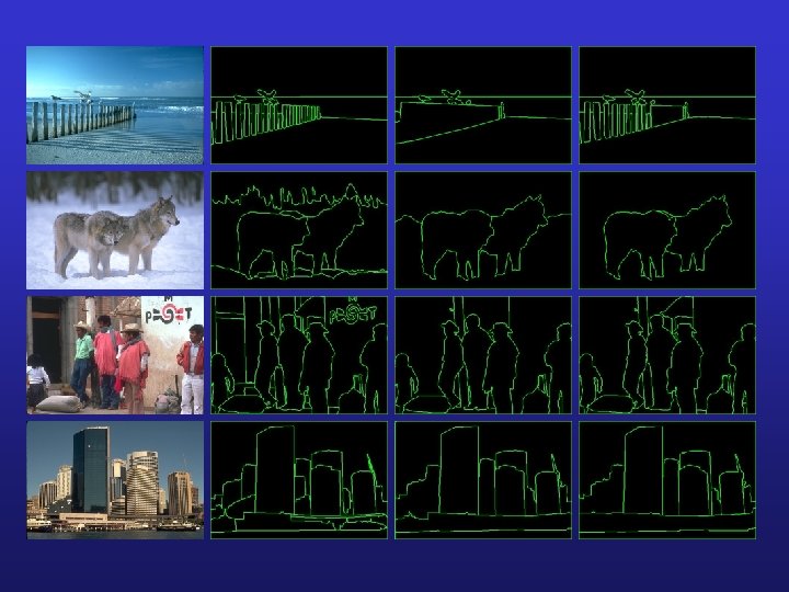
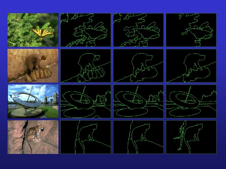
Segmentations are not identical

But are they consistent?

Perceptual organization produces a hierarchy image background grass bush far left bird beak eye right bird head body eye head body Each subject picks a cross section from this hierarchy

Quantifying inconsistency. . How much is segmentation S 1 a refinement of segmentation S 2 at pixel pi? S 1 refinement of S 2 E(S 1, S 2, pi) = |(R(S 1, pi)R(S 2, pi)| |R(S 1, pi)|

Segmentation Error Measure • One-way Local Refinement Error: LRE(S 1, S 2, pi) = ||(R(S 1, pi) R(S 2, pi)|| ||R(S 1, pi)|| • Segmentation Error defined to allow refinement in either direction at each pixel: SE(S 1, S 2) = 1/n i min {LRE(S 1, S 2, pi), LRE(S 2, S 1, pi)}

Distribution of SE over Dataset

Gray, Color, Inv. Neg Datasets • Explore how various high/low-level cues affect the task of image segmentation by subjects – Color = full color image – Gray = luminance image – Inv. Neg = inverted negative luminance image

Color Gray Inv. Neg

Inv. Neg

Color Gray Inv. Neg

Gray vs. Color vs. Inv. Neg Segmentations SE (gray, gray) = 0. 047 SE (gray, color) = 0. 047 SE (gray, invneg) = 0. 059 • Color may affect attention, but doesn’t seem to affect perceptual organization • Inv. Neg seems to interfere with high-level cues 2500 gray segmentations 2500 color segmentations 200 invneg segmentations

Outline of talk • Creating a dataset of human segmented images • Measuring ecological statistics of various Gestalt grouping factors • Using these measurements to calibrate and validate approaches to grouping

Natural images aren’t generic signals • Filter statistics are far from Gaussian. . – Ruderman 1994, 1997 – Field, Olshausen 1996 – Huang, Mumford 1999, 2000 – Buccigrossi, Simoncelli 1999 • These properties (e. g. scale-invariance, sparsity, heavy tails) can be exploited for image compression.

P (Same. Segment | Proximity)

P (Same. Segment | Luminance)

Quantifying the power of cues • Bayes Risk • Mutual information

Bayes Risk for Proximity Cue

Mutual information where x is a cue and y is indicator of being in same segment

Bayes Risk for Various Cues Given Proximity

Mutual Information for Various Cues Given Proximity

Power of various cues Bayes Mutual Risk Info. Proximity 0. 335 0. 044 Luminance 0. 369 0. 016 Color 0. 369 0. 014 Intervening 0. 303 Contour Texture 0. 300 0. 081 0. 112

Spatial priors on image regions and contours

Distribution of Region Area y = Kx- = 0. 913

Distribution of length • Decompose contours at high curvature extrema

Distribution of Length

Distribution of Length Slope = 2. 05 in Log-Log Plot I. e, frequency 1 / ( length )^2 ( for region area it’s roughly 1/area )

Conditioned on Region Size

Scale invariance of contour statistics • Chi-square distance 0 0. 0409 0. 0538 0. 0409 0 0. 0531 0 0. 0538

Marginal Distribution of Curvature

Distribution of Region Convexity

Outline of talk • Creating a dataset of human segmented images • Measuring ecological statistics of various Gestalt grouping factors • Using these measurements to calibrate and validate approaches to grouping

Computational Mechanisms for Visual Grouping Jitendra Malik, Serge Belongie, Jianbo Shi, Thomas Leung U. C. Berkeley

Edge-based image segmentation • Edge detection by gradient operators • Linking by dynamic programming, voting, relaxation, … Montanari 71, Parent&Zucker 89, Guy&Medioni 96, Shaashua&Ullman 88 Williams&Jacobs 95, Geiger&Kumaran 96, Heitger&von der Heydt 93 - Natural for encoding curvilinear grouping Hard decisions often made prematurely Produce meaningless clutter in textured regions

Edges in textured regions are meaningless clutter image orientation energy

Region-based image segmentation • 1970 s produced region growing, split-and-merge, etc. . . • 1980 s led to approaches based on a global criterion for image segmentation – Markov Random Fields e. g. Geman&Geman 84 – Variational approaches e. g. Mumford&Shah 89 – Expectation-Maximization e. g. Ayer&Sawhney 95, Weiss 97 • Global method, but computational complexity precludes exact MAP estimation – Curvilinear grouping not easily enforced – Unable to handle line-drawings – Problems due to local minima

Our Approach • Global decision good, local bad – Formulate as hierarchical graph partitioning • Efficient computation – Draw on ideas from spectral graph theory to define an eigenvalue problem which can be solved for finding segmentation. • Develop suitable encoding of visual cues in terms of graph weights.

Image Segmentation as Graph Partitioning Build a weighted graph G=(V, E) from image V: image pixels E: connections between pairs of nearby pixels Partition graph so that similarity within group is large and similarity between groups is small -- Normalized Cuts [Shi&Malik 97]

Normalized Cuts as a Spring-Mass system • Each pixel is a point mass; each connection is a spring: • Fundamental modes are generalized eigenvectors of

Some Terminology for Graph Partitioning • How do we bipartition a graph:

Normalized Cut, A measure of dissimilarity • Minimum cut is not appropriate since it favors cutting small pieces. • Normalized Cut, Ncut:

Normalized Cut and Normalized Association • Minimizing similarity between the groups, and maximizing similarity within the groups can be achieved simultaneously.

Solving the Normalized Cut problem • Exact discrete solution to Ncut is NPcomplete even on regular grid, – [Papadimitriou’ 97] • Drawing on spectral graph theory, good approximation can be obtained by solving a generalized eigenvalue problem.

Some definitions

Normalized Cut As Generalized Eigenvalue problem • Rewriting Normalized Cut in matrix form:

More math…

Normalized Cut As Generalized Eigenvalue problem • after simplification, we get

Normalized Cut As Generalized Eigenvalue problem • The eigenvector with the second smallest eigenvalue of the generalized eigensystem: • is the solution to the constrained Raleigh quotient:

Interpretation as a Dynamical System • The equivalent spring-mass system: • The generalized eigenvectors are the fundamental modes of oscillation.

Video

Computational Aspects • Solving for the generalized eigensystem: • (D-W) is of size , but it is sparse with O(N) nonzero entries, where N is the number of pixels. • Using Lanczos algorithm.

Overall Procedure • Construct a weighted graph G=(V, E) from an image • Connect each pair of pixels, and assign graph edge weight, • Solve for the smallest few eigenvectors, • Recursively subdivide if Ncut value is below a prespecified value.

Normalized Cuts Approach • Global decision good, local bad – Formulate as hierarchical graph partitioning • Efficient computation – Draw on ideas from spectral graph theory to define an eigenvalue problem which can be solved for finding segmentation. • Develop suitable encoding of visual cues in terms of graph weights.

Cue Integration • based on Texton histograms • based on Intervening contour •

Filters for Texture Description • Elongated directional Gaussian derivatives • 2 nd derivative and Hilbert transform • L 1 normalized for scale invariance • 6 orientations, 3 scales • Zero mean

Textons • K-means on vectors of filter responses

Textons (cont. )

Benefits of the Texton Representation • Discrete point sets well suited to tools of computational geometry, point process statistics • Defining Local Scale Selection • Measuring Texture Similarity

Texton Histograms Chi square test: i j k 0. 1 0. 8

Intervening Contours as and are more likely to belong to the same region than are and.

Estimating Image for contour cue Orientation Energy • Estimate where is the maximum orientation energy along segment ij

Orientation Energy • Gaussian 2 nd derivative and its Hilbert pair • • Can detect combination of bar and edge features; also insensitive to linear shading [Perona&Malik 90] • Multiple scales

Challenges of Cue Integration • Contour cue tends to fragment textured regions • Texture cue tends to create 1 D regions from contours

Texture as a problem for contour processing image orientation energy

Contour as a problem for texture processing Segmentation based on Gaussian Mixture Model EM

Cue Integration • Gate contour vs. texture cue based on region -boundary vs. region-interior label • Compute boundary vs. interior label using statistical test on region uniformity • Multiply to get combined weight:

Motion Segmentation with Normalized Cuts • Networks of spatial-temporal connections:

Motion Segmentation with Normalized Cuts • Motion “proto-volume” in space-time • Group correspondence

Results • video

Results

Results

Stereoscopic data

Framework for Recognition (1) Segmentation Pixels Segments Over-segmentation necessary; Undersegmentation fatal (2) Association Segments Regions Enumerate: # of size k regions in image with n segments is ~(4**k)*n/k (3) Matching Regions Prototypes ~10 views/object. Matching tolerant to pose/illumination changes, intra-category variation, error in previous steps