TopDown approaches to the NACP an overview Steven

Top-Down approaches to the NACP: an overview Steven C. Wofsy, Harvard University Daniel M. Matross, UC Berkeley Colorado Springs, January, 2007 University of Wyoming King Air approaches the NOAA-ESRL tall tower at Argyle, ME, June, 2004.

What is a Top-Down analysis… in the NACP? Top-down analysis derives surface fluxes over North America, and sub-regions of North America from atmospheric observations of concentrations of carbon gases (CO 2, CH 4) in the atmosphere. Variations in time and space are caused by inputs and outputs at the surface, acted upon by air motions. If a limited area (e. g. North America or a region) is the target, variable boundary conditions add complexity. Strengths of the top-down: integral constraints are applied, obtaining integrated fluxes. Scalable in both space and time. Bottom-up analysis derives surface fluxes from small-scale models of the underlying biogeochemistry for each patch of land, driven by weather, season, etc. Strengths of the bottom-up: verifiable fluxes, with relationship to underlying causes Top-down models are inverse models: observed variations in the atmosphere (emergent properties) are analyzed to infer the underlying fluxes (causation).

The inconvenient truths about top-down models • It is not possible to uniquely determine the budget on regional scales from atmospheric observations. The top-down modeling problem is intrinsically under-constrained. • We need them: they are the only means to obtaining credible regional and continental budgets of CO 2, CO, and CH 4. There are many sensitivities in the results from top-down models that are not readily incorporated into an inverse-model framework, but which can provide dominant sources of bias and stochastic errors.

Top-down models are usually thought to have very limited need for a detailed bottom-up model fluxes—large areas are typically aggregated in global inverse models, while a variety of simple surface flux models are used for more regional studies. This represents a false dichotomy between top-down and bottom-up models. Since top-down models are under-constrained, information from the assumed pattern of fluxes survives into the final budget estimates. Thus top-down models require very careful design of the surface flux field to be optimized against data. The underlying reason is that observations are influenced by fluxes at all spatial scales, including the near field and the global field, and everything in between. There are many other features and design elements of top-down models that can affect the results…

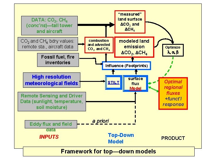
“measured” land surface DCO 2 and DCH 4 DATA: CO 2, CH 4 (conc'ns)—tall tower and aircraft CO 2 and CH 4 bdry values: remote sta. , aircraft data Fossil fuel, fire inventories High resolution meteorological fields combustion and advected CO 2 and CH 4 modeled land emission DCO 2, DCH 4 INPUTS , a, b Influence (Footprints) STILT surface flux Model Remote Sensing and Driver Data (sunlight, temperature, soil moisture) Eddy flux and field data Optimize Optimal regional fluxes +funct'l response a priori Top-Down Model Framework for top—down models PRODUCT

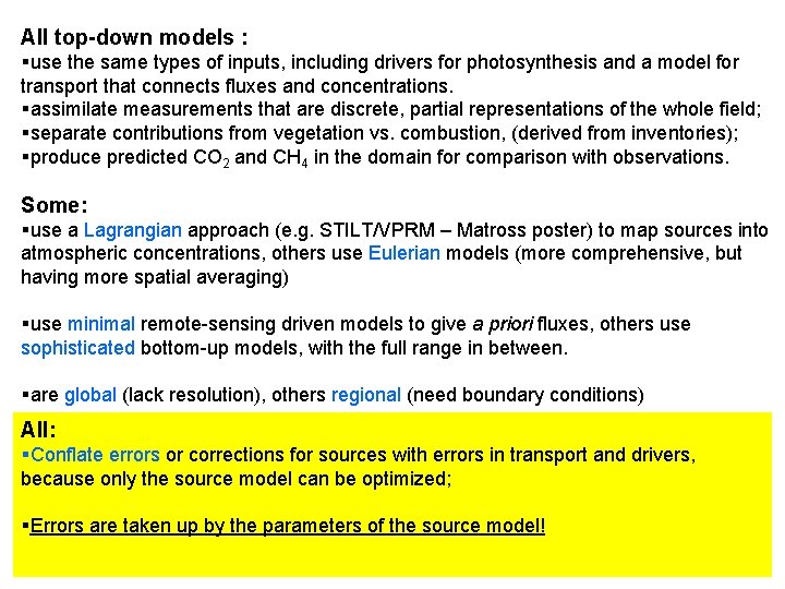
All top-down models : §use the same types of inputs, including drivers for photosynthesis and a model for transport that connects fluxes and concentrations. §assimilate measurements that are discrete, partial representations of the whole field; §separate contributions from vegetation vs. combustion, (derived from inventories); §produce predicted CO 2 and CH 4 in the domain for comparison with observations. Some: §use a Lagrangian approach (e. g. STILT/VPRM – Matross poster) to map sources into atmospheric concentrations, others use Eulerian models (more comprehensive, but having more spatial averaging) §use minimal remote-sensing driven models to give a priori fluxes, others use sophisticated bottom-up models, with the full range in between. §are global (lack resolution), others regional (need boundary conditions) All: §Conflate errors or corrections for sources with errors in transport and drivers, because only the source model can be optimized; §Errors are taken up by the parameters of the source model!

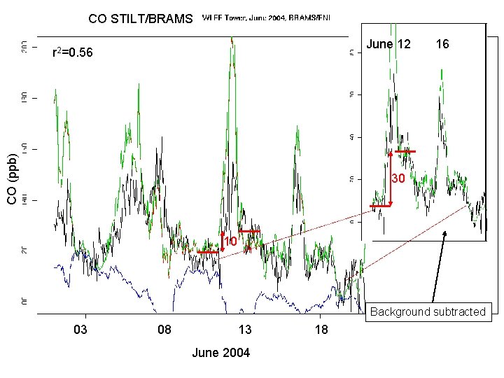
Example: Conflated corrections to source strengths/budgets with errors in transport. The role of the boundary in regional analysis Illustrated by modeling of CO data at WLEF. Domain (45 km, BRAMS) = all of North America, from the Arctic to the tropics, Feb. 2004—Jan 2005.

CO STILT/BRAMS June 12 16 CO (ppb) r 2=0. 56 30 10 Background subtracted 03 08 13 18 June 2004

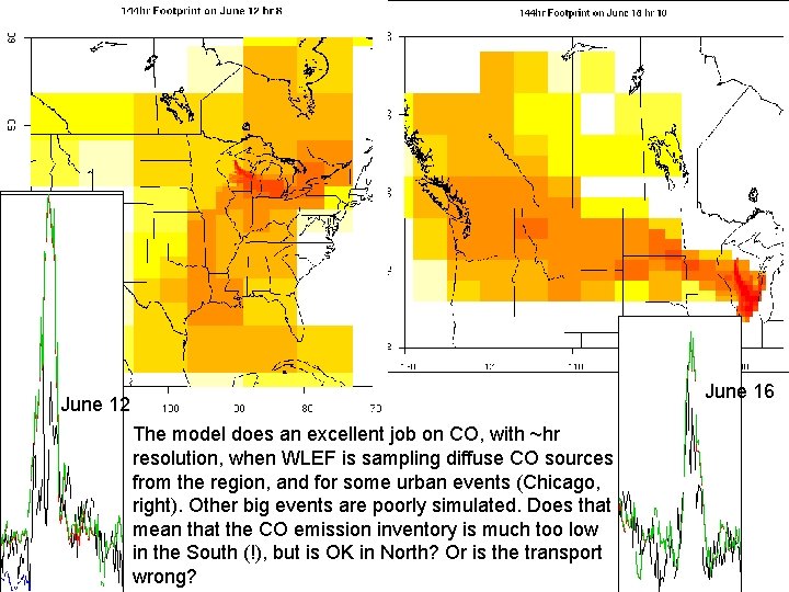
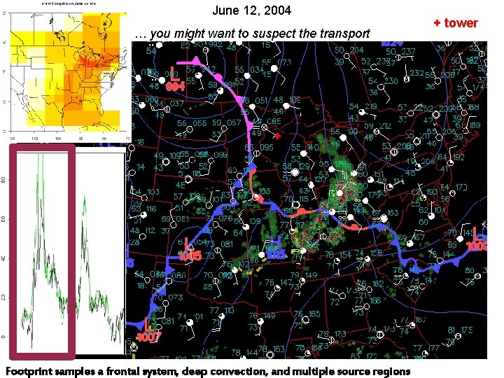
June 16 June 12 The model does an excellent job on CO, with ~hr resolution, when WLEF is sampling diffuse CO sources from the region, and for some urban events (Chicago, right). Other big events are poorly simulated. Does that mean that the CO emission inventory is much too low in the South (!), but is OK in North? Or is the transport wrong?

June 12, 2004 … you might want to suspect the transport + Footprint samples a frontal system, deep convection, and multiple source regions + tower

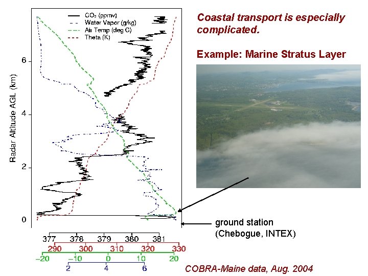
Coastal transport is especially complicated. Example: Marine Stratus Layer ground station (Chebogue, INTEX) COBRA-Maine data, Aug. 2004

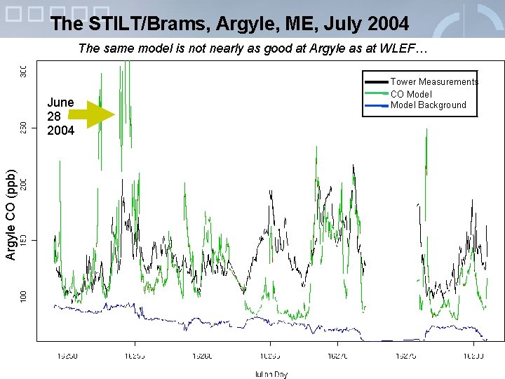
The STILT/Brams, Argyle, ME, July 2004 The same model is not nearly as good at Argyle as at WLEF… Argyle CO (ppb) June 28 2004 Tower Measurements CO Model Background

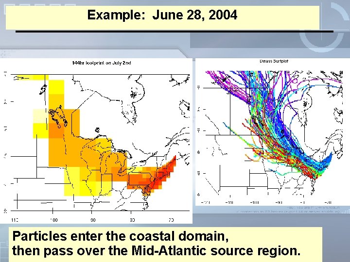
Example: June 28, 2004 Particles enter the coastal domain, then pass over the Mid-Atlantic source region.

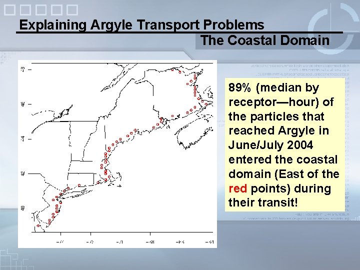
Explaining Argyle Transport Problems The Coastal Domain 89% (median by receptor—hour) of the particles that reached Argyle in June/July 2004 entered the coastal domain (East of the red points) during their transit!

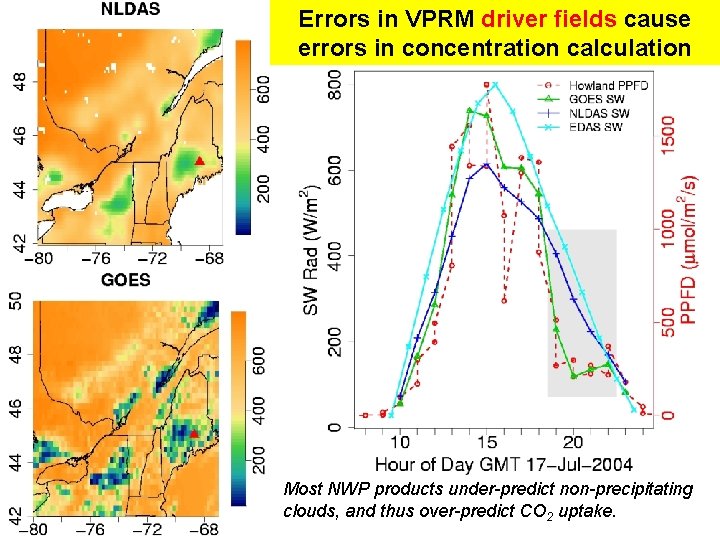
Errors in VPRM driver fields cause errors in concentration calculation Most NWP products under-predict non-precipitating clouds, and thus over-predict CO 2 uptake.

The Way Forward

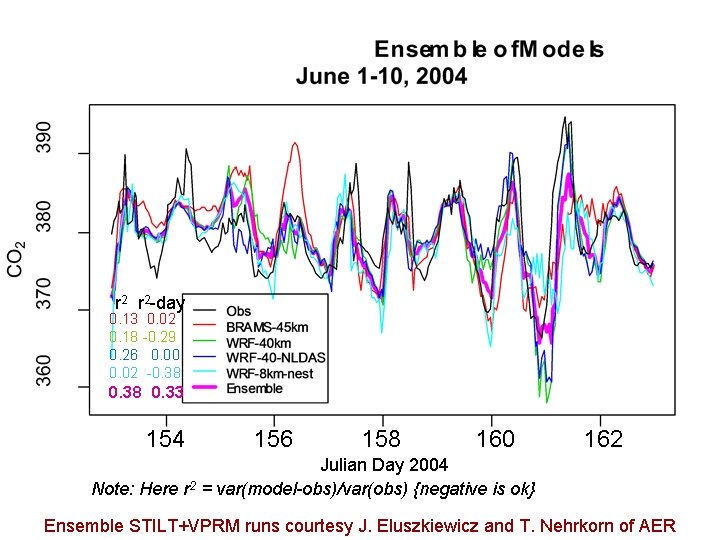
r 2 r 2 -day 0. 13 0. 02 0. 18 -0. 29 0. 26 0. 00 0. 02 -0. 38 0. 33 154 156 158 160 162 Julian Day 2004 Note: Here r 2 = var(model-obs)/var(obs) {negative is ok} Ensemble STILT+VPRM runs courtesy J. Eluszkiewicz and T. Nehrkorn of AER

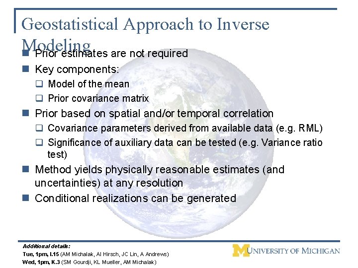
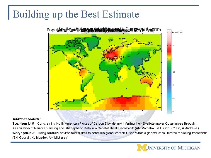
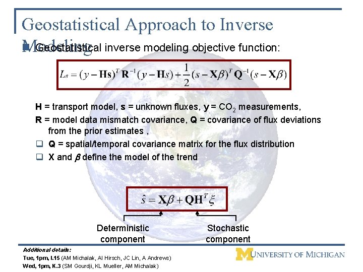
Geostatistical Approach to Inverse Modeling n Prior estimates are not required n Key components: q Model of the mean q Prior covariance matrix n Prior based on spatial and/or temporal correlation q Covariance parameters derived from available data (e. g. RML) q Significance of auxiliary data can be tested (e. g. Variance ratio test) n Method yields physically reasonable estimates (and uncertainties) at any resolution n Conditional realizations can be generated Additional details: Tue, 1 pm, I. 15 (AM Michalak, AI Hirsch, JC Lin, A Andrews) Wed, 1 pm, K. 3 (SM Gourdji, KL Mueller, AM Michalak)

Building up the Best Estimate Additional details: Tue, 1 pm, I. 15: Constraining North American Fluxes of Carbon Dioxide and Inferring their Spatiotemporal Covariances through Assimilation of Remote Sensing and Atmospheric Data in a Geostatistical Framework (AM Michalak, AI Hirsch, JC Lin, A Andrews) Wed, 1 pm, K. 3: Using auxiliary environmental data to constrain global carbon fluxes within a geostatistical inverse modeling framework (SM Gourdji, KL Mueller, AM Michalak)

The basic framework for regional and continental inverse modeling is well understood, even as the implementation remains subject to major scientific issues. Utilizing this framework in an operational program has its own major challenges. The Global Monitoring Division of NOAA ESRL has initiated a program to begin operational diagnostic analysis of the North American Carbon Program: Carbon. Tracker P. Tans and W. Peters starting their new project. New ESRL equipment item… CO 2 ?

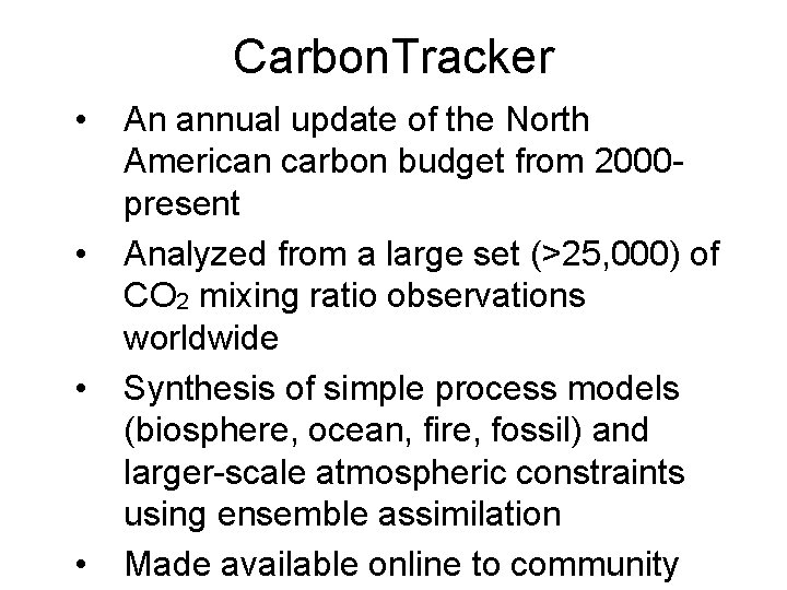
Carbon. Tracker • • An annual update of the North American carbon budget from 2000 present Analyzed from a large set (>25, 000) of CO 2 mixing ratio observations worldwide Synthesis of simple process models (biosphere, ocean, fire, fossil) and larger-scale atmospheric constraints using ensemble assimilation Made available online to community

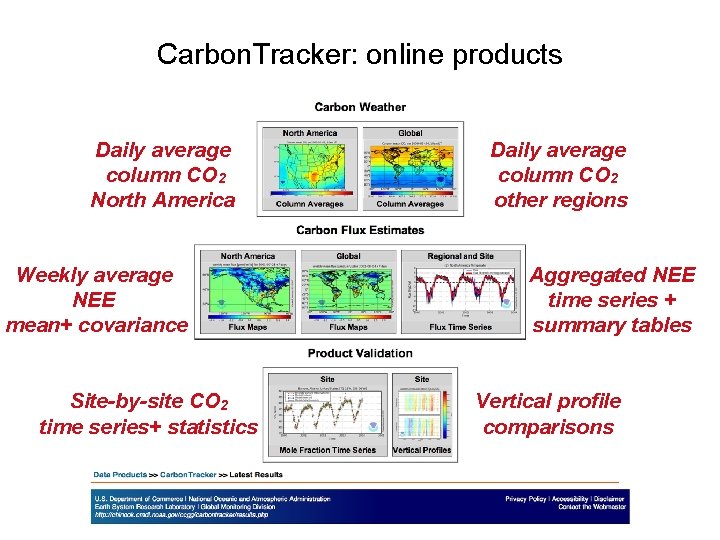
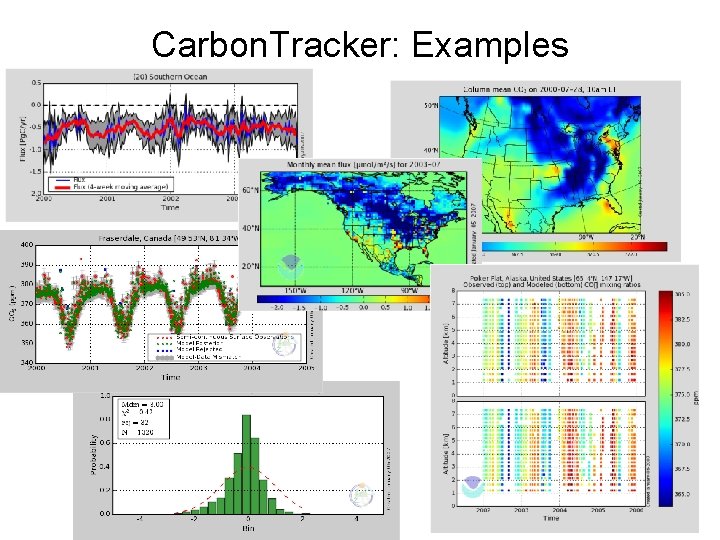
Carbon. Tracker: online products Daily average column CO 2 North America Weekly average NEE mean+ covariance Site-by-site CO 2 time series+ statistics Daily average column CO 2 other regions Aggregated NEE time series + summary tables Vertical profile comparisons

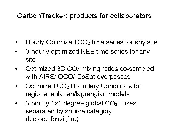
Carbon. Tracker: products for collaborators • • • Hourly Optimized CO 2 time series for any site 3 -hourly optimized NEE time series for any site Optimized 3 D CO 2 mixing ratios co-sampled with AIRS/ OCO/ Go. Sat overpasses Optimized CO 2 Boundary Conditions for regional eularian/lagrangian models 3 -hourly 1 x 1 degree global CO 2 fluxes separated by source category (bio, oce, fossil, fire)

Carbon. Tracker: Examples

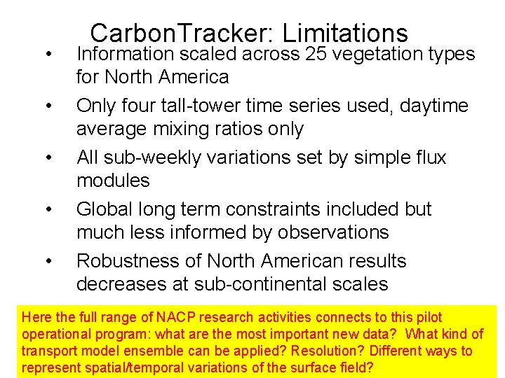
• • • Carbon. Tracker: Limitations Information scaled across 25 vegetation types for North America Only four tall-tower time series used, daytime average mixing ratios only All sub-weekly variations set by simple flux modules Global long term constraints included but much less informed by observations Robustness of North American results decreases at sub-continental scales Here the full range of NACP research activities connects to this pilot operational program: what are the most important new data? What kind of transport model ensemble can be applied? Resolution? Different ways to represent spatial/temporal variations of the surface field?

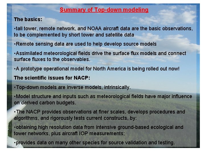
Summary of Top-down modeling The basics: • tall tower, remote network, and NOAA aircraft data are the basic observations, to be complemented by short tower and satellite data • Remote sensing data are used to help develop source models • Assimilated meteorological fields drive the surface flux models and connect surface fluxes to the observables. • A prototype operational model for North America is being rolled out now! The scientific issues for NACP: • Top-down models are inverse models, intrinsically. • Model structure and inputs such as meteorological fields have major influence on derived carbon budgets. • The NACP provides observations at finer scales, develops procedures and algorithms, and rigorously tests current constructs, by: • obtaining high resolution data from intensive ground-based ecological and tower networks, plus aircraft IOP measurements; • provides data on many other species for source validation and testing.

What are the current challenges for top-down modeling? Driver data – sunshine, meteorology, phenology Surface source model(s)--spatial and temporal resolution, accuracy, scalability Transport models--mass conservation, mixed layer, "boundary values", internal boundaries (coast) Inversion procedures--bias, transport error, covariances, dimensionality, selection of most significant additional data.

Thanks to all those who contributed data, slides, and ideas (very many people!)

SLIDES NOT IN USE

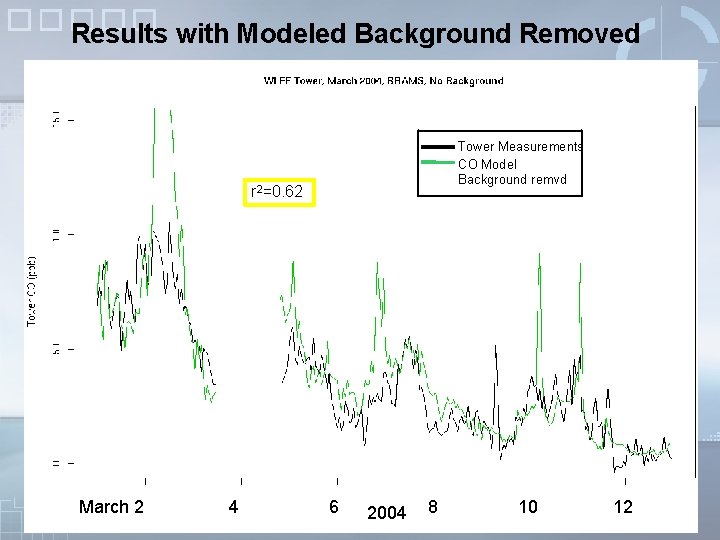
Results with Modeled Background Removed r 2=0. 62 Tower Measurements CO Model Background remvd March 2 4 6 8 10 12 2004

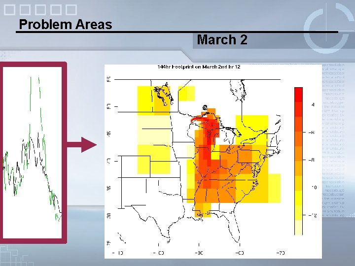
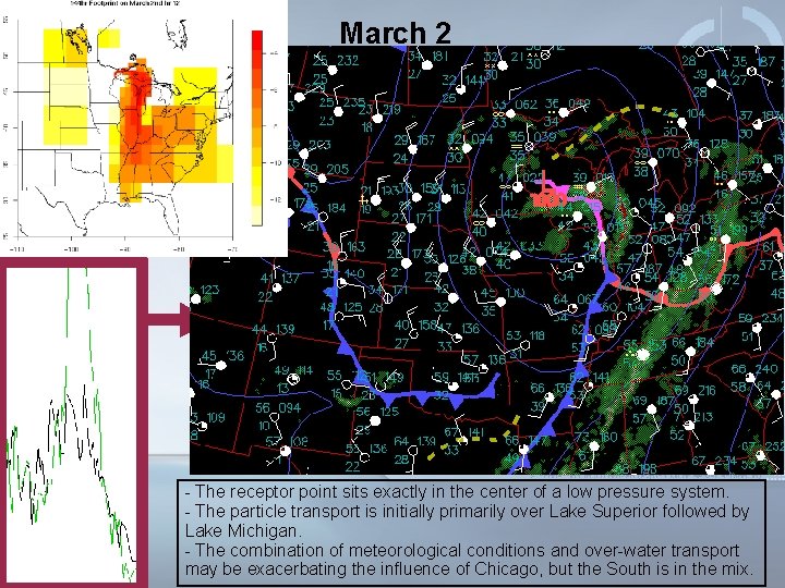
Problem Areas March 2

Problem Areas March 2 - The receptor point sits exactly in the center of a low pressure system. - The particle transport is initially primarily over Lake Superior followed by Lake Michigan. - The combination of meteorological conditions and over-water transport may be exacerbating the influence of Chicago, but the South is in the mix.

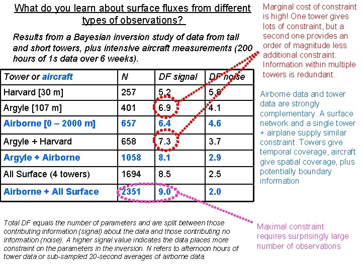
What do you learn about surface fluxes from different types of observations? Results from a Bayesian inversion study of data from tall and short towers, plus intensive aircraft measurements (200 hours of 1 s data over 6 weeks). Tower or aircraft N DF signal DF noise Harvard [30 m] 257 5. 2 5. 8 Argyle [107 m] 401 6. 9 4. 1 Airborne [0 – 2000 m] 657 6. 4 4. 6 Argyle + Harvard 658 7. 3 3. 7 Argyle + Airborne 1058 8. 1 2. 9 All Surface (4 towers) 1694 8. 5 2. 5 Airborne + All Surface 2351 9. 0 2. 0 Total DF equals the number of parameters and are split between those contributing information (signal) about the data and those contributing no information (noise). A higher signal value indicates the data places more constraint on the parameters in the inversion. N refers to afternoon hours of tower data or sub-sampled 20 -second averages of airborne data. Marginal cost of constraint is high! One tower gives lots of constraint, but a second one provides an order of magnitude less additional constraint. Information within multiple towers is redundant. Airborne data and tower data are strongly complementary. A surface network and a single tower + airplane supply similar constraint. Towers give temporal coverage, aircraft give spatial coverage, plus potentially boundary information Maximal constraint requires surprisingly large number of observations

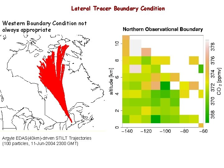
Lateral Tracer Boundary Condition Western Boundary Condition not always appropriate Argyle EDAS(40 km)-driven STILT Trajectories {100 particles, 11 -Jun-2004 2300 GMT}

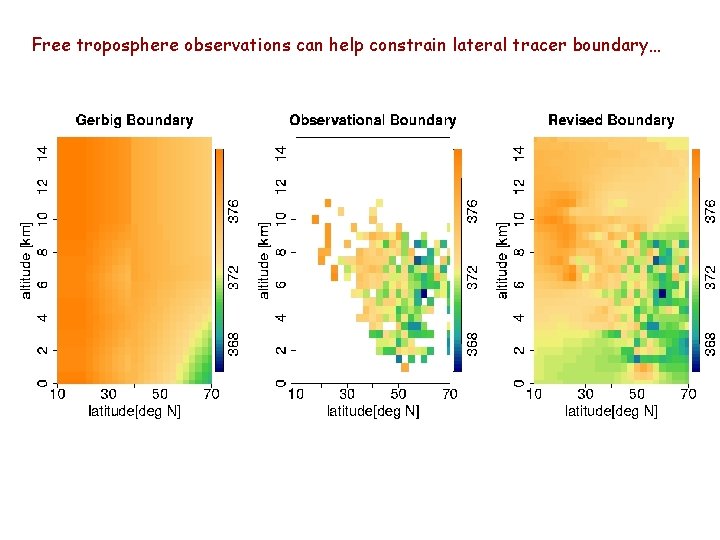
Free troposphere observations can help constrain lateral tracer boundary…

Geostatistical Approach to Inverse n Geostatistical inverse modeling objective function: Modeling H = transport model, s = unknown fluxes, y = CO 2 measurements, R = model data mismatch covariance, Q = covariance of flux deviations from the prior estimates , q Q = spatial/temporal covariance matrix for the flux distribution q X and define the model of the trend Deterministic component Additional details: Tue, 1 pm, I. 15 (AM Michalak, AI Hirsch, JC Lin, A Andrews) Wed, 1 pm, K. 3 (SM Gourdji, KL Mueller, AM Michalak) Stochastic component