Statistics and Data Analysis Professor William Greene Stern

Statistics and Data Analysis Professor William Greene Stern School of Business IOMS Department of Economics 1/54 2: Descriptive Statistics

Statistics and Data Analysis Part 2 – Descriptive Statistics Summarizing data with useful statistics 2/54 2: Descriptive Statistics

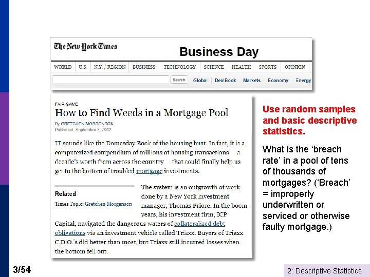
Use random samples and basic descriptive statistics. What is the ‘breach rate’ in a pool of tens of thousands of mortgages? (‘Breach’ = improperly underwritten or serviced or otherwise faulty mortgage. ) 3/54 2: Descriptive Statistics

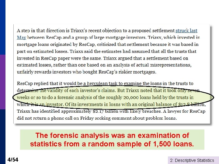
The forensic analysis was an examination of statistics from a random sample of 1, 500 loans. 4/54 2: Descriptive Statistics

Descriptive Statistics Agenda Populations and Random Samples p Descriptive Statistics for a Variable p n n p Measuring Correlation of Two Variables n n n 5/54 Measures of location: Mean, median, mode Measure of dispersion: Standard deviation Understanding correlation Measuring correlation Scatter plots and regression 2: Descriptive Statistics

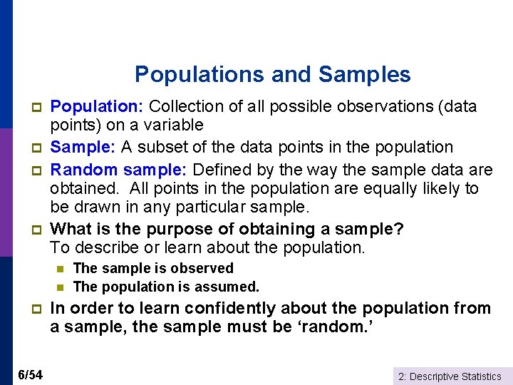
Populations and Samples p p Population: Collection of all possible observations (data points) on a variable Sample: A subset of the data points in the population Random sample: Defined by the way the sample data are obtained. All points in the population are equally likely to be drawn in any particular sample. What is the purpose of obtaining a sample? To describe or learn about the population. n n p 6/54 The sample is observed The population is assumed. In order to learn confidently about the population from a sample, the sample must be ‘random. ’ 2: Descriptive Statistics

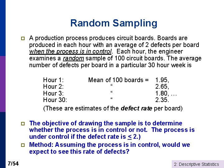
Random Sampling p A production process produces circuit boards. Boards are produced in each hour with an average of 2 defects per board when the process is in control. Each hour, the engineer examines a random sample of 100 circuit boards. The average number of defects per board in a particular 30 hour week is Hour 1: Mean of 100 boards = 1. 95, Hour 2: “ 2. 65, Hour 3: “ 1. 80, … Hour 30: “ 2. 35. (These are estimates of the defect rate per board) p p 7/54 The objective of drawing the sample is to determine whether the process is in control or not. The process is under control if the defect rate is < 2. ) Method: Assuming the process is in control, would we expect to see this rate of defects? 2: Descriptive Statistics

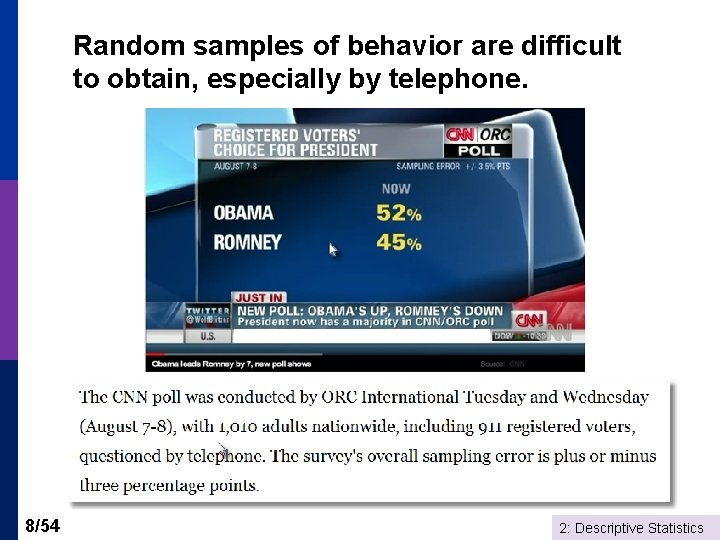
Random samples of behavior are difficult to obtain, especially by telephone. 8/54 2: Descriptive Statistics

Nonrandom Samples Nonrandom samples produce tainted, sometimes not believable results n n 9/54 Biased with respect to the population May describe a not useful specific subset of the population. 2: Descriptive Statistics

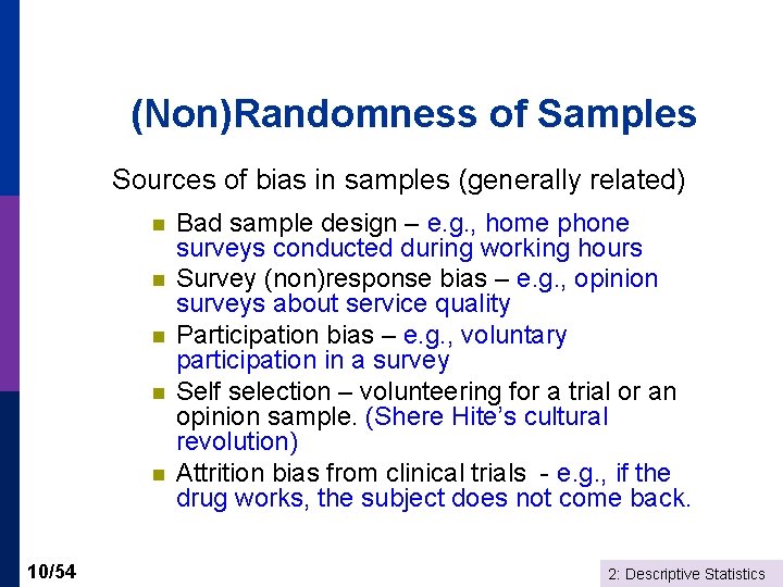
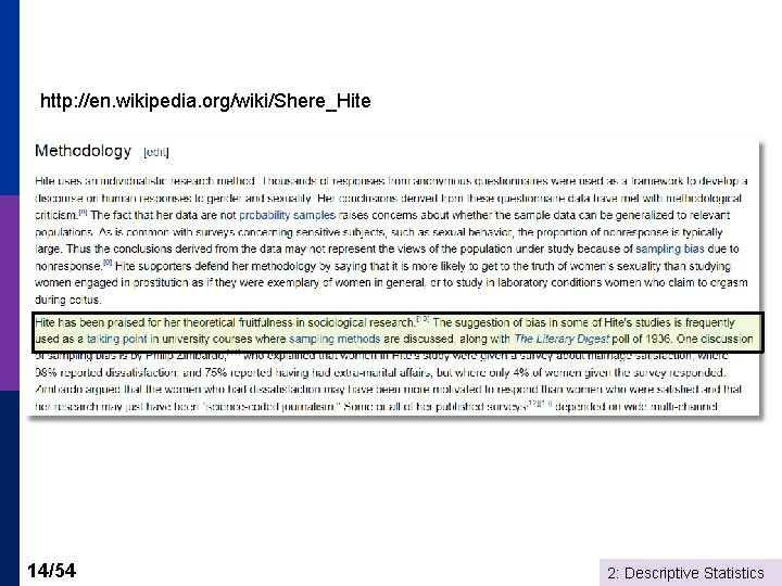
(Non)Randomness of Samples Sources of bias in samples (generally related) n n n 10/54 Bad sample design – e. g. , home phone surveys conducted during working hours Survey (non)response bias – e. g. , opinion surveys about service quality Participation bias – e. g. , voluntary participation in a survey Self selection – volunteering for a trial or an opinion sample. (Shere Hite’s cultural revolution) Attrition bias from clinical trials - e. g. , if the drug works, the subject does not come back. 2: Descriptive Statistics

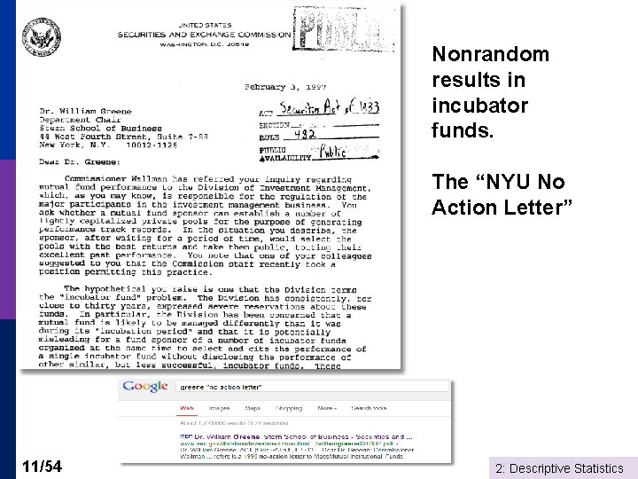
Nonrandom results in incubator funds. The “NYU No Action Letter” 11/54 2: Descriptive Statistics

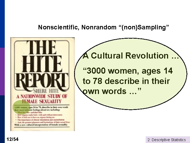
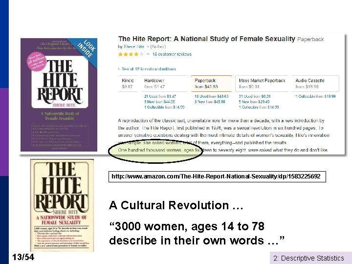
Nonscientific, Nonrandom “(non)Sampling” A Cultural Revolution … “ 3000 women, ages 14 to 78 describe in their own words …” 12/54 2: Descriptive Statistics

http: //www. amazon. com/The-Hite-Report-National-Sexuality/dp/1583225692 A Cultural Revolution … “ 3000 women, ages 14 to 78 describe in their own words …” 13/54 2: Descriptive Statistics

http: //en. wikipedia. org/wiki/Shere_Hite 14/54 2: Descriptive Statistics

The Lesson… Having a really big sample does not assure you of an accurate result. It may assure you of a really solid, really bad (inaccurate) result. 15/54 2: Descriptive Statistics

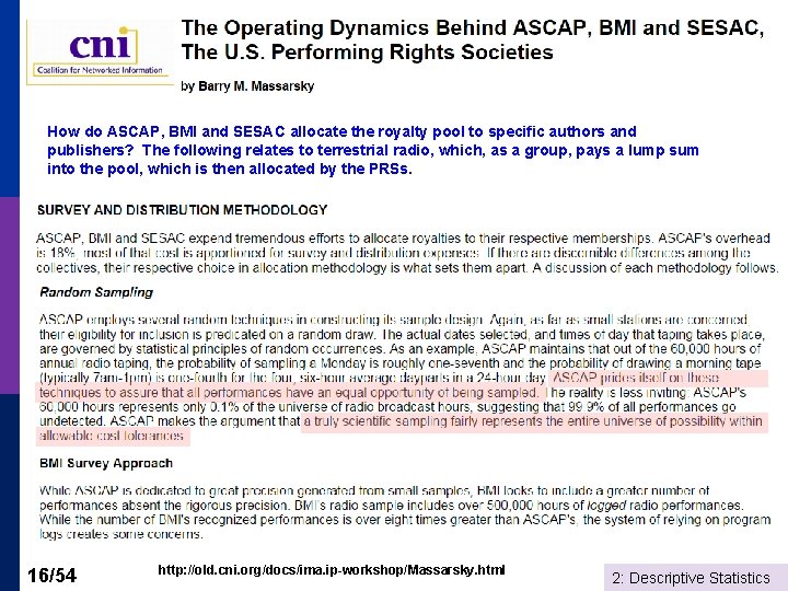
How do ASCAP, BMI and SESAC allocate the royalty pool to specific authors and publishers? The following relates to terrestrial radio, which, as a group, pays a lump sum into the pool, which is then allocated by the PRSs. 16/54 http: //old. cni. org/docs/ima. ip-workshop/Massarsky. html 2: Descriptive Statistics

A Descriptive Statistic Is … ? p Describes what? p n The sample data n The population that the data came from 17/54 2: Descriptive Statistics

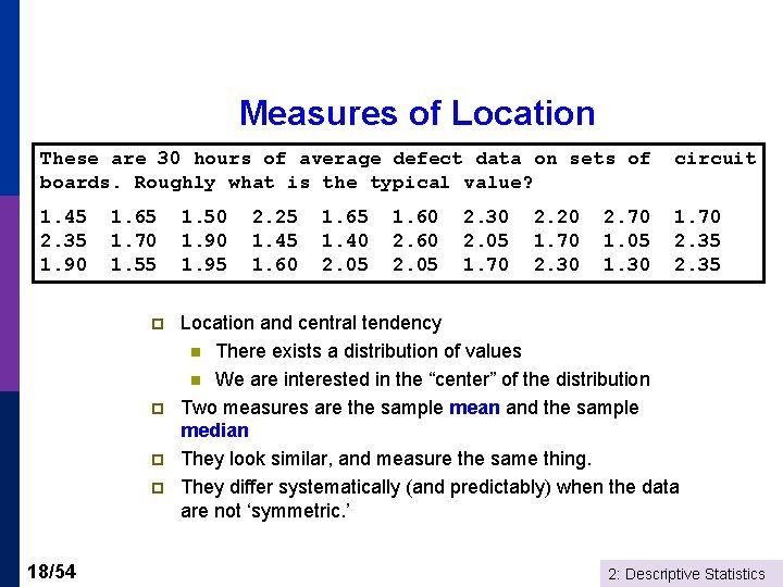
Measures of Location These are 30 hours of average defect data on sets of boards. Roughly what is the typical value? circuit 1. 45 2. 35 1. 90 1. 70 2. 35 1. 65 1. 70 1. 55 p p 18/54 1. 50 1. 95 2. 25 1. 45 1. 60 1. 65 1. 40 2. 05 1. 60 2. 05 2. 30 2. 05 1. 70 2. 20 1. 70 2. 30 2. 70 1. 05 1. 30 Location and central tendency n There exists a distribution of values n We are interested in the “center” of the distribution Two measures are the sample mean and the sample median They look similar, and measure the same thing. They differ systematically (and predictably) when the data are not ‘symmetric. ’ 2: Descriptive Statistics

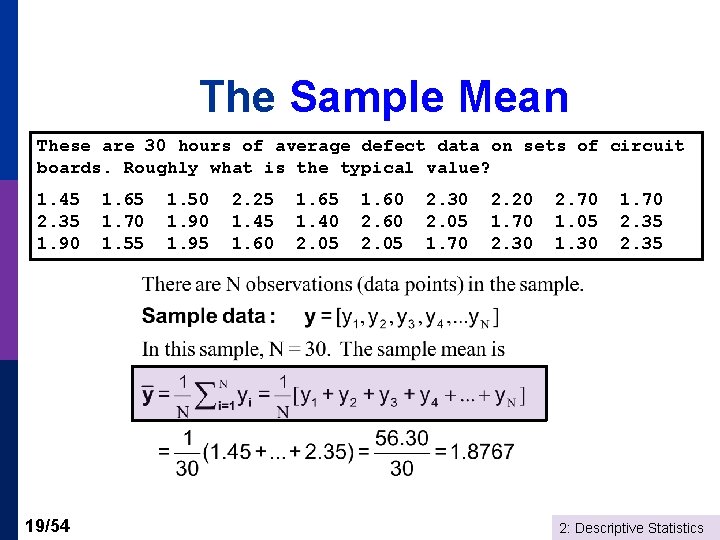
The Sample Mean These are 30 hours of average defect data on sets of circuit boards. Roughly what is the typical value? 1. 45 2. 35 1. 90 19/54 1. 65 1. 70 1. 55 1. 50 1. 95 2. 25 1. 45 1. 60 1. 65 1. 40 2. 05 1. 60 2. 05 2. 30 2. 05 1. 70 2. 20 1. 70 2. 30 2. 70 1. 05 1. 30 1. 70 2. 35 2: Descriptive Statistics

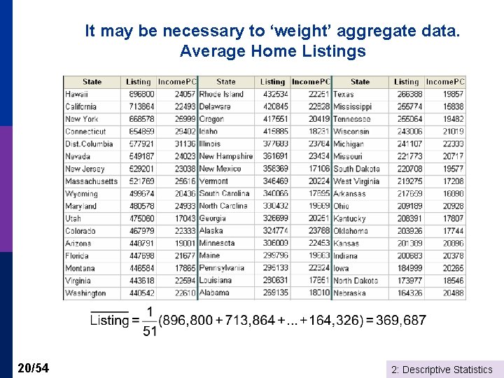
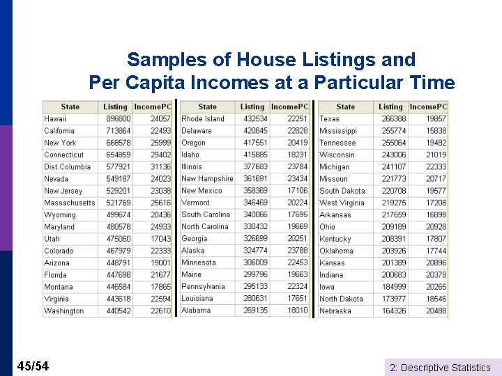
It may be necessary to ‘weight’ aggregate data. Average Home Listings 20/54 2: Descriptive Statistics

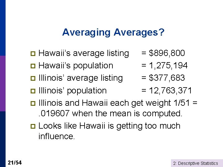
Averaging Averages? Hawaii’s average listing = $896, 800 p Hawaii’s population = 1, 275, 194 p Illinois’ average listing = $377, 683 p Illinois’ population = 12, 763, 371 p Illinois and Hawaii each get weight 1/51 =. 019607 when the mean is computed. p Looks like Hawaii is getting too much influence. p 21/54 2: Descriptive Statistics

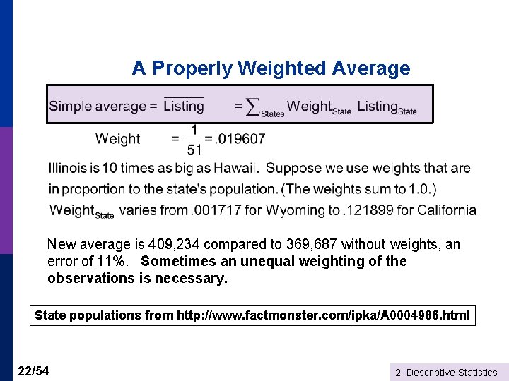
A Properly Weighted Average New average is 409, 234 compared to 369, 687 without weights, an error of 11%. Sometimes an unequal weighting of the observations is necessary. State populations from http: //www. factmonster. com/ipka/A 0004986. html 22/54 2: Descriptive Statistics

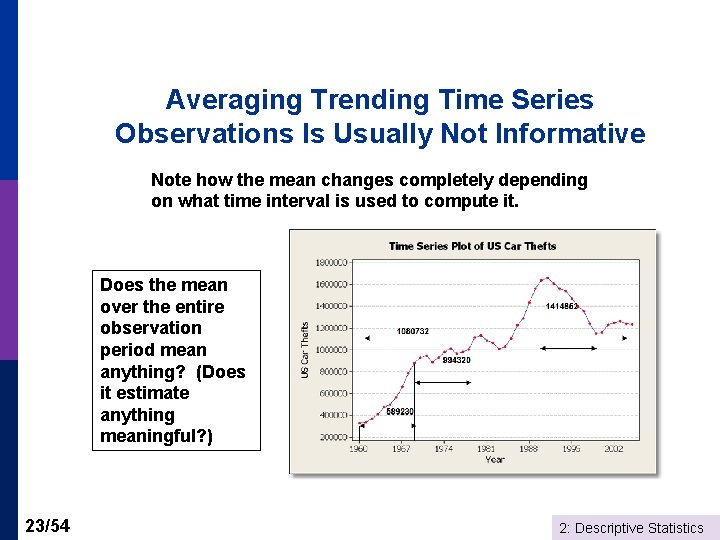
Averaging Trending Time Series Observations Is Usually Not Informative Note how the mean changes completely depending on what time interval is used to compute it. Does the mean over the entire observation period mean anything? (Does it estimate anything meaningful? ) 23/54 2: Descriptive Statistics

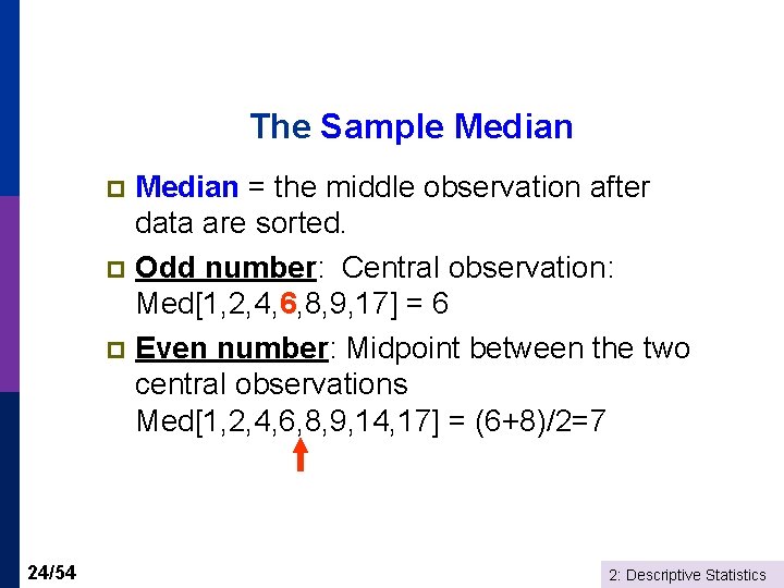
The Sample Median = the middle observation after data are sorted. p Odd number: Central observation: Med[1, 2, 4, 6, 8, 9, 17] = 6 p Even number: Midpoint between the two central observations Med[1, 2, 4, 6, 8, 9, 14, 17] = (6+8)/2=7 p 24/54 2: Descriptive Statistics

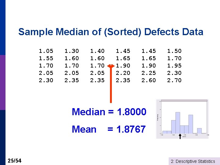
Sample Median of (Sorted) Defects Data 1. 05 1. 55 1. 70 2. 05 2. 30 1. 60 1. 70 2. 05 2. 35 1. 40 1. 60 1. 70 2. 05 2. 35 1. 45 1. 65 1. 90 2. 20 2. 35 1. 45 1. 65 1. 90 2. 25 2. 60 1. 50 1. 70 1. 95 2. 30 2. 70 Median = 1. 8000 Mean 25/54 = 1. 8767 2: Descriptive Statistics

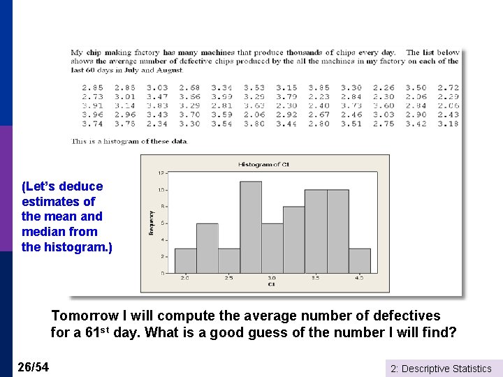
(Let’s deduce estimates of the mean and median from the histogram. ) Tomorrow I will compute the average number of defectives for a 61 st day. What is a good guess of the number I will find? 26/54 2: Descriptive Statistics

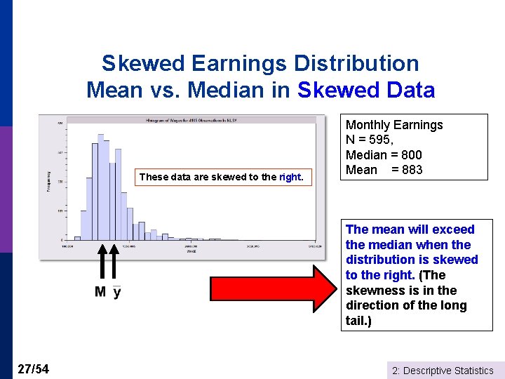
Skewed Earnings Distribution Mean vs. Median in Skewed Data These data are skewed to the right. Monthly Earnings N = 595, Median = 800 Mean = 883 The mean will exceed the median when the distribution is skewed to the right. (The skewness is in the direction of the long tail. ) 27/54 2: Descriptive Statistics

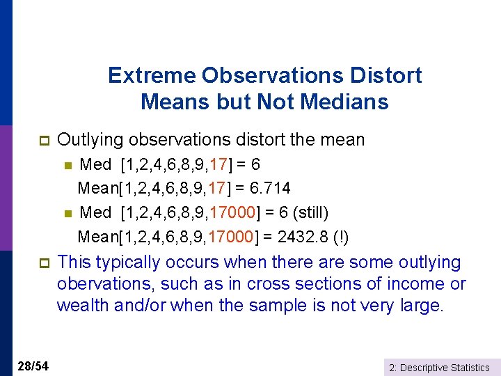
Extreme Observations Distort Means but Not Medians p Outlying observations distort the mean Med [1, 2, 4, 6, 8, 9, 17] = 6 Mean[1, 2, 4, 6, 8, 9, 17] = 6. 714 n Med [1, 2, 4, 6, 8, 9, 17000] = 6 (still) Mean[1, 2, 4, 6, 8, 9, 17000] = 2432. 8 (!) n p 28/54 This typically occurs when there are some outlying obervations, such as in cross sections of income or wealth and/or when the sample is not very large. 2: Descriptive Statistics

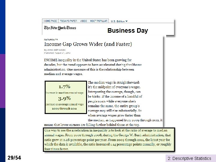
29/54 2: Descriptive Statistics

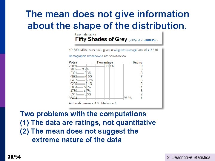
The mean does not give information about the shape of the distribution. Two problems with the computations (1) The data are ratings, not quantitative (2) The mean does not suggest the extreme nature of the data 30/54 2: Descriptive Statistics

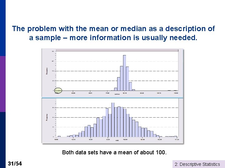
The problem with the mean or median as a description of a sample – more information is usually needed. Both data sets have a mean of about 100. 31/54 2: Descriptive Statistics

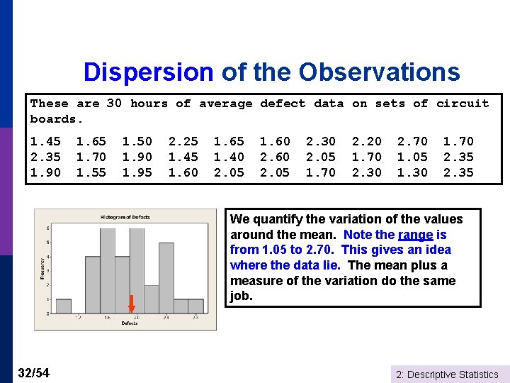
Dispersion of the Observations These are 30 hours of average defect data on sets of circuit boards. 1. 45 2. 35 1. 90 1. 65 1. 70 1. 55 1. 50 1. 95 2. 25 1. 45 1. 60 1. 65 1. 40 2. 05 1. 60 2. 05 2. 30 2. 05 1. 70 2. 20 1. 70 2. 30 2. 70 1. 05 1. 30 1. 70 2. 35 We quantify the variation of the values around the mean. Note the range is from 1. 05 to 2. 70. This gives an idea where the data lie. The mean plus a measure of the variation do the same job. 32/54 2: Descriptive Statistics

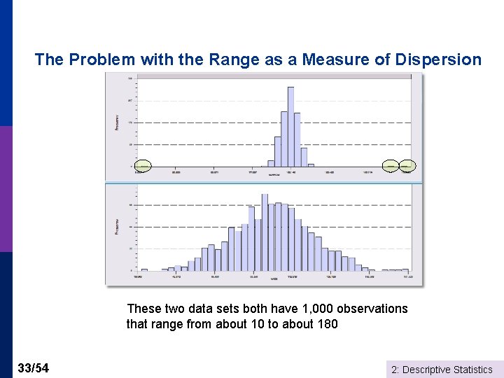
The Problem with the Range as a Measure of Dispersion These two data sets both have 1, 000 observations that range from about 10 to about 180 33/54 2: Descriptive Statistics

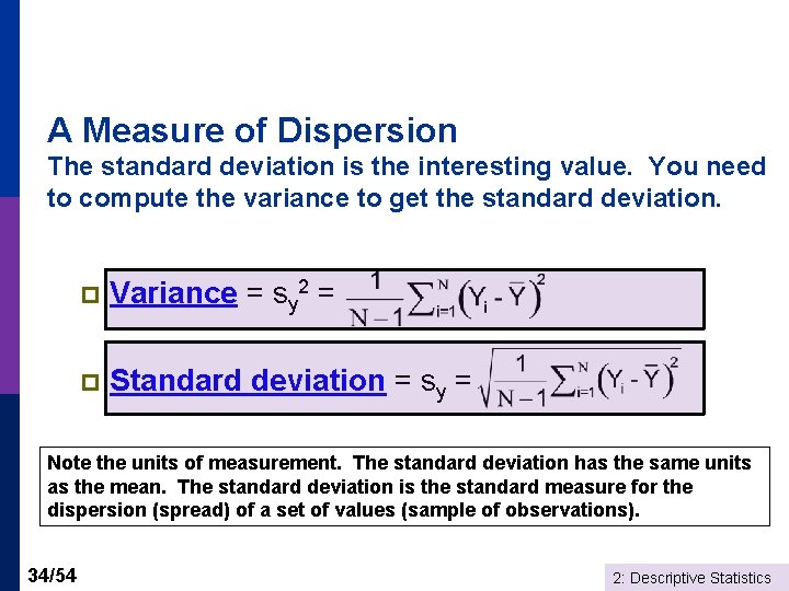
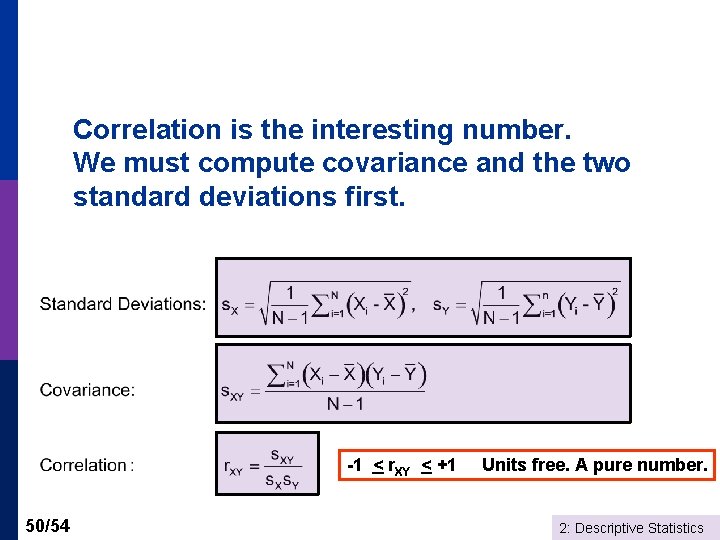
A Measure of Dispersion The standard deviation is the interesting value. You need to compute the variance to get the standard deviation. p Variance = sy 2 = p Standard deviation = sy = Note the units of measurement. The standard deviation has the same units as the mean. The standard deviation is the standard measure for the dispersion (spread) of a set of values (sample of observations). 34/54 2: Descriptive Statistics

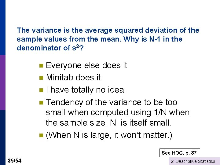
The variance is the average squared deviation of the sample values from the mean. Why is N-1 in the denominator of s 2? Everyone else does it n Minitab does it n I have totally no idea. n Tendency of the variance to be too small when computed using 1/N when the sample size, N, is itself small. n (When N is large, it won’t matter. ) n See HOG, p. 37 35/54 2: Descriptive Statistics

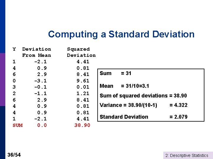
Computing a Standard Deviation Y Deviation From Mean 1 -2. 1 4 0. 9 6 2. 9 0 -3. 1 3 -0. 1 2 -1. 1 6 2. 9 4 0. 9 1 -2. 1 SUM 0. 0 36/54 Squared Deviation 4. 41 0. 81 8. 41 9. 61 0. 01 1. 21 8. 41 0. 81 4. 41 38. 90 Sum = 31 Mean = 31/10=3. 1 Sum of squared deviations = 38. 90 Variance = 38. 90/(10 -1) = 4. 322 Standard Deviation = 2. 079 2: Descriptive Statistics

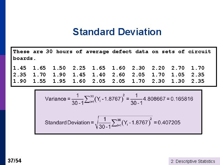
Standard Deviation These are 30 hours of average defect data on sets of circuit boards. 1. 45 2. 35 1. 90 37/54 1. 65 1. 70 1. 55 1. 50 1. 95 2. 25 1. 45 1. 60 1. 65 1. 40 2. 05 1. 60 2. 05 2. 30 2. 05 1. 70 2. 20 1. 70 2. 30 2. 70 1. 05 1. 30 1. 70 2. 35 2: Descriptive Statistics

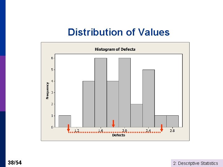
Distribution of Values 38/54 2: Descriptive Statistics

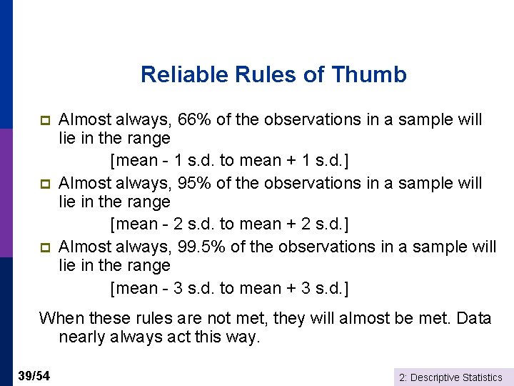
Reliable Rules of Thumb p p p Almost always, 66% of the observations in a sample will lie in the range [mean - 1 s. d. to mean + 1 s. d. ] Almost always, 95% of the observations in a sample will lie in the range [mean - 2 s. d. to mean + 2 s. d. ] Almost always, 99. 5% of the observations in a sample will lie in the range [mean - 3 s. d. to mean + 3 s. d. ] When these rules are not met, they will almost be met. Data nearly always act this way. 39/54 2: Descriptive Statistics

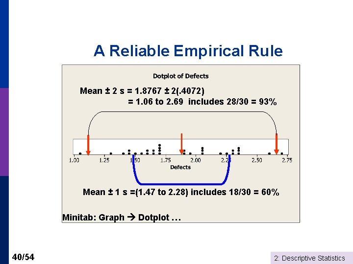
A Reliable Empirical Rule Mean ± 2 s = 1. 8767 ± 2(. 4072) = 1. 06 to 2. 69 includes 28/30 = 93% Mean ± 1 s =(1. 47 to 2. 28) includes 18/30 = 60% Minitab: Graph Dotplot … 40/54 2: Descriptive Statistics

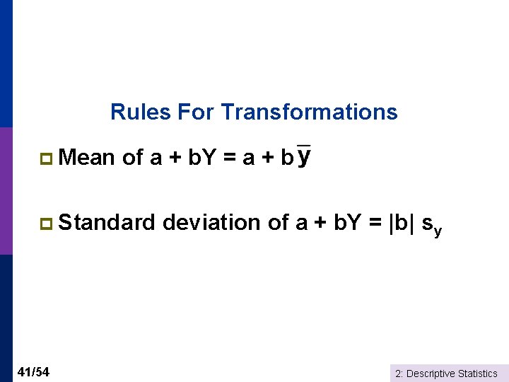
Rules For Transformations p Mean of a + b. Y = a + b p Standard 41/54 deviation of a + b. Y = |b| sy 2: Descriptive Statistics

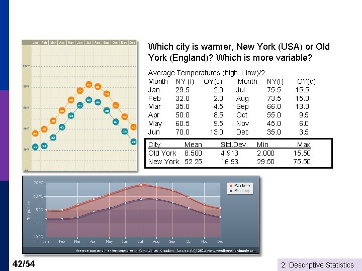
Which city is warmer, New York (USA) or Old York (England)? Which is more variable? Average Temperatures (high + low)/2 Month NY (f) OY(c) Month Jan 29. 5 2. 0 Jul Feb 32. 0 Aug Mar 35. 0 4. 5 Sep Apr 50. 0 8. 5 Oct May 60. 5 9. 5 Nov Jun 70. 0 13. 0 Dec City Mean Old York 8. 500 New York 52. 25 42/54 Std. Dev. 4. 913 16. 93 NY(f) 75. 5 73. 5 66. 0 55. 0 45. 0 35. 0 Min 2. 000 29. 50 OY(c) 15. 5 15. 0 13. 0 9. 5 6. 0 3. 5 Max 15. 50 75. 50 2: Descriptive Statistics

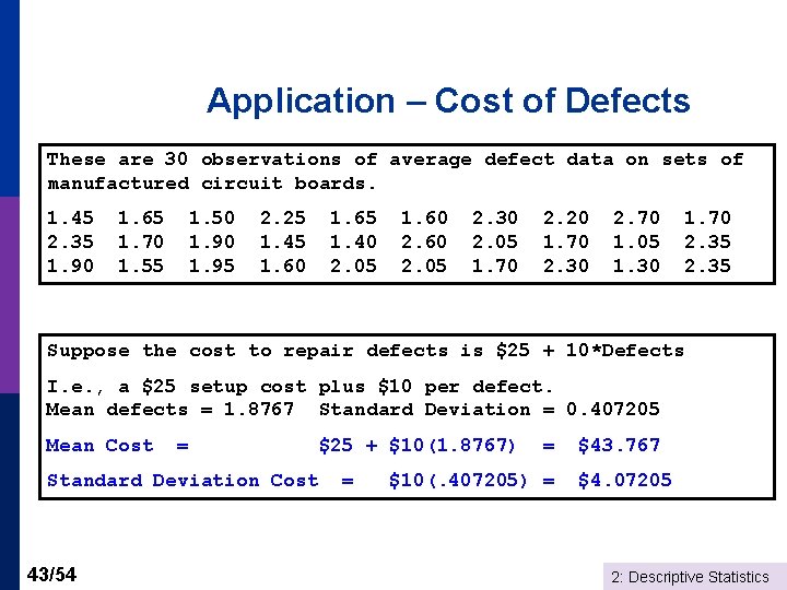
Application – Cost of Defects These are 30 observations of average defect data on sets of manufactured circuit boards. 1. 45 2. 35 1. 90 1. 65 1. 70 1. 55 1. 50 1. 95 2. 25 1. 45 1. 60 1. 65 1. 40 2. 05 1. 60 2. 05 2. 30 2. 05 1. 70 2. 20 1. 70 2. 30 2. 70 1. 05 1. 30 1. 70 2. 35 Suppose the cost to repair defects is $25 + 10*Defects I. e. , a $25 setup cost plus $10 per defect. Mean defects = 1. 8767 Standard Deviation = 0. 407205 Mean Cost = Standard Deviation Cost 43/54 $25 + $10(1. 8767) = = $10(. 407205) = $43. 767 $4. 07205 2: Descriptive Statistics

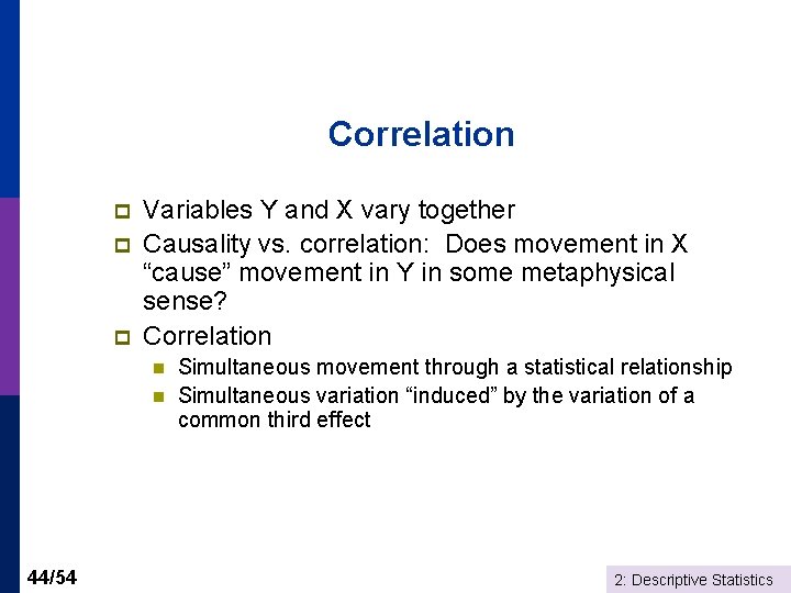
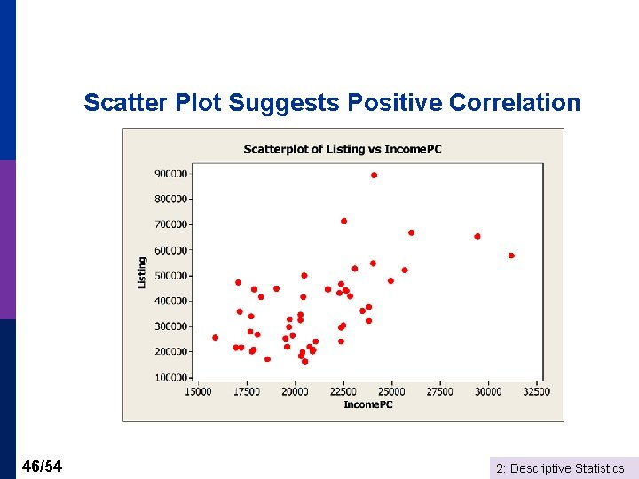
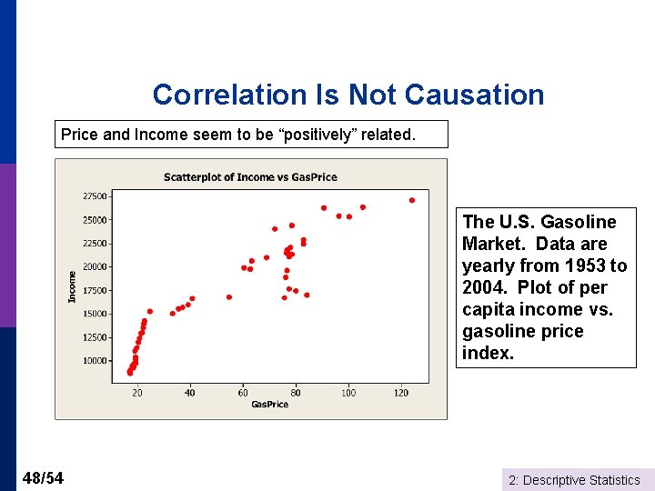
Correlation p p p Variables Y and X vary together Causality vs. correlation: Does movement in X “cause” movement in Y in some metaphysical sense? Correlation n n 44/54 Simultaneous movement through a statistical relationship Simultaneous variation “induced” by the variation of a common third effect 2: Descriptive Statistics

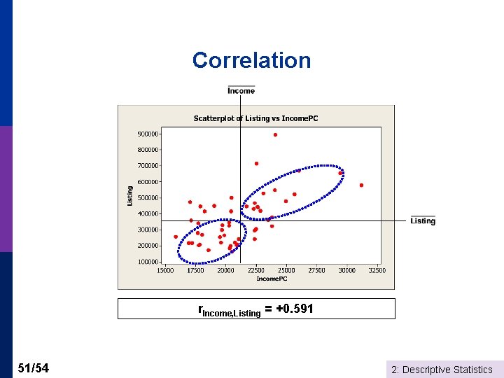
Samples of House Listings and Per Capita Incomes at a Particular Time 45/54 2: Descriptive Statistics

Scatter Plot Suggests Positive Correlation 46/54 2: Descriptive Statistics

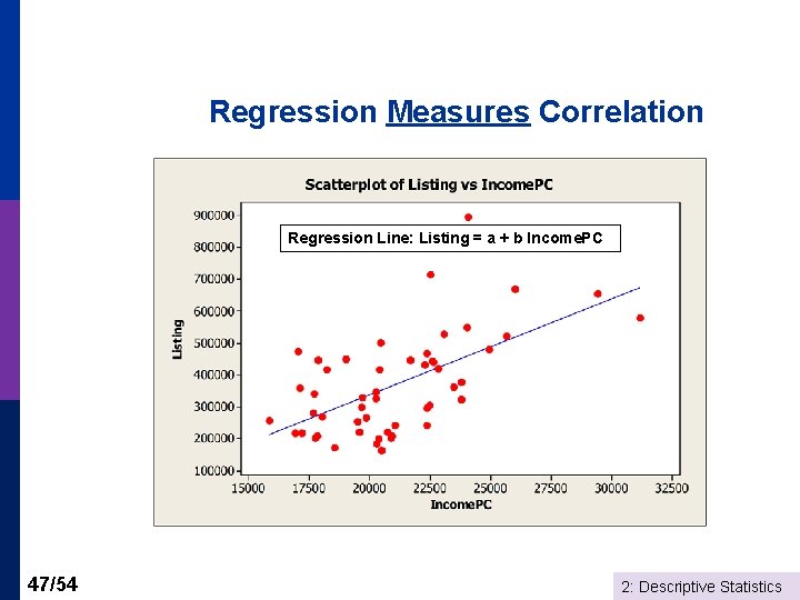
Regression Measures Correlation Regression Line: Listing = a + b Income. PC 47/54 2: Descriptive Statistics

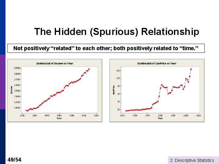
Correlation Is Not Causation Price and Income seem to be “positively” related. The U. S. Gasoline Market. Data are yearly from 1953 to 2004. Plot of per capita income vs. gasoline price index. 48/54 2: Descriptive Statistics

The Hidden (Spurious) Relationship Not positively “related” to each other; both positively related to “time. ” 49/54 2: Descriptive Statistics

Correlation is the interesting number. We must compute covariance and the two standard deviations first. -1 < r. XY < +1 50/54 Units free. A pure number. 2: Descriptive Statistics

Correlation r. Income, Listing = +0. 591 51/54 2: Descriptive Statistics

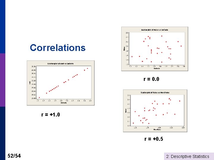
Correlations r = 0. 0 r = +1. 0 r = +0. 5 52/54 2: Descriptive Statistics

Sample Statistics and Population Parameters p p p 53/54 Sample has a sample mean and standard deviation and s. Y. Population has a mean, μ, and standard deviation, σ. The sample “looks like” the population. The sample statistics resemble the population features. The bigger is the RANDOM sample, the closer will be the resemblance. We will study this later in the course. 2: Descriptive Statistics

Summary p Statistics to describe location (mean) and spread (standard deviation) of a sample of values. n n n p Statistics and graphical tools to describe bivariate (two variable) relationships n n 54/54 Interpretations Computations Complications Scatter plots Correlation 2: Descriptive Statistics