Statistics and Data Analysis Professor William Greene Stern

Statistics and Data Analysis Professor William Greene Stern School of Business IOMS Department of Economics 1/46 Part 12: Statistical Inference

Statistics and Data Analysis Part 12 – Statistical Inference: Confidence Intervals 2/46 Part 12: Statistical Inference

3/46 Part 12: Statistical Inference

Statistical Inference: Point Estimates and Confidence Intervals p p Statistical Inference Estimation of Population Features Using Sample Data Sampling Distributions of Statisticss Point Estimates and the Law of Large Numbers n n 4/46 Uncertainty in Estimation Interval Estimation Part 12: Statistical Inference

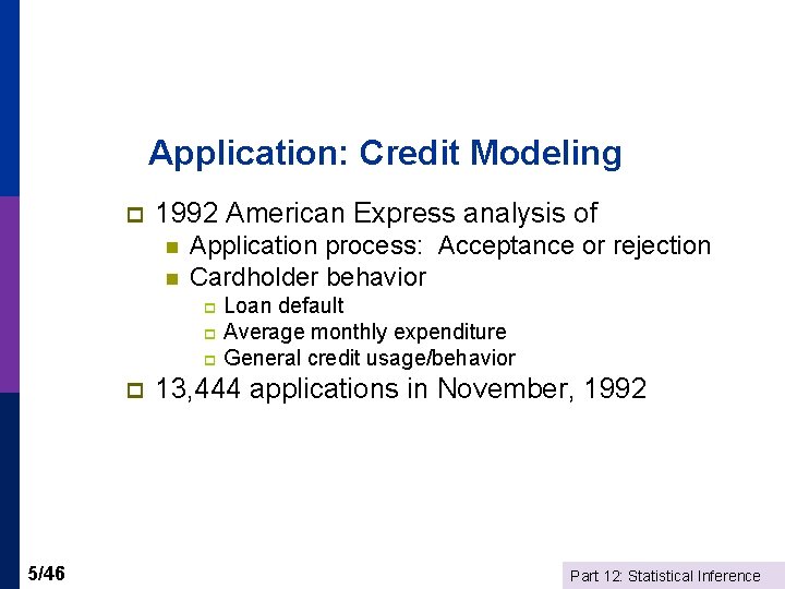
Application: Credit Modeling p 1992 American Express analysis of n n Application process: Acceptance or rejection Cardholder behavior Loan default p Average monthly expenditure p General credit usage/behavior p p 5/46 13, 444 applications in November, 1992 Part 12: Statistical Inference

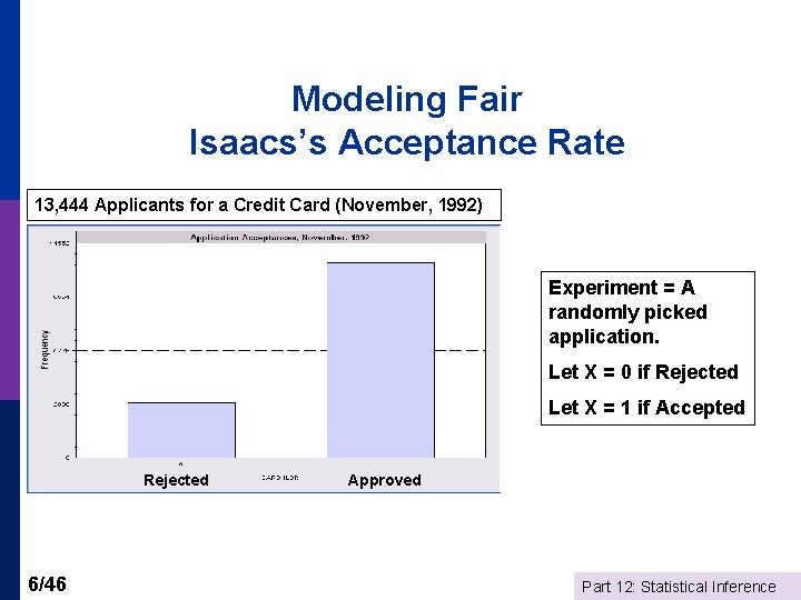
Modeling Fair Isaacs’s Acceptance Rate 13, 444 Applicants for a Credit Card (November, 1992) Experiment = A randomly picked application. Let X = 0 if Rejected Let X = 1 if Accepted Rejected 6/46 Approved Part 12: Statistical Inference

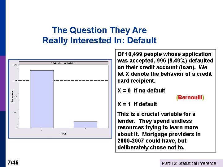
The Question They Are Really Interested In: Default Of 10, 499 people whose application was accepted, 996 (9. 49%) defaulted on their credit account (loan). We let X denote the behavior of a credit card recipient. X = 0 if no default (Bernoulli) X = 1 if default This is a crucial variable for a lender. They spend endless resources trying to learn more about it. Mortgage providers in 2000 -2007 could have, but deliberately chose not to. 7/46 Part 12: Statistical Inference

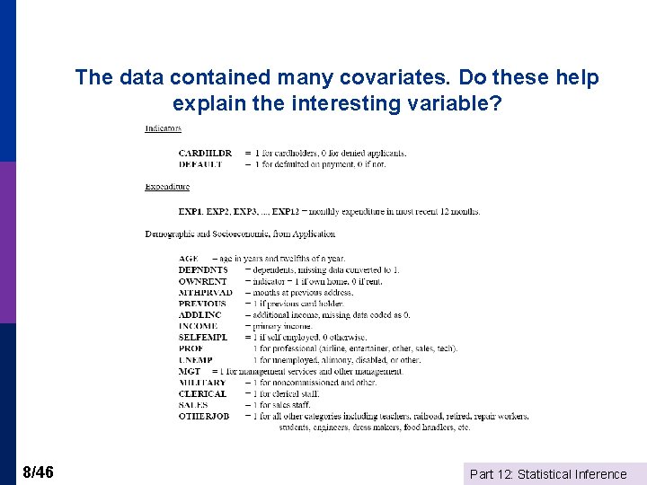
The data contained many covariates. Do these help explain the interesting variable? 8/46 Part 12: Statistical Inference

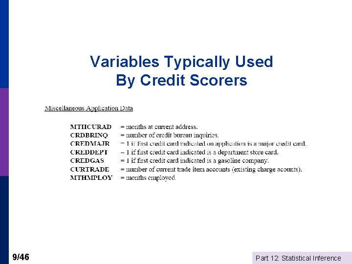
Variables Typically Used By Credit Scorers 9/46 Part 12: Statistical Inference

Sample Statistics p The population has characteristics n n n p 10/46 Mean, variance Median Percentiles A random sample is a “slice” of the population Part 12: Statistical Inference

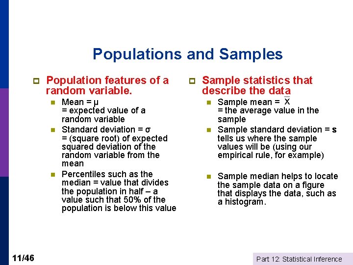
Populations and Samples p Population features of a random variable. n n n 11/46 Mean = μ = expected value of a random variable Standard deviation = σ = (square root) of expected squared deviation of the random variable from the mean Percentiles such as the median = value that divides the population in half – a value such that 50% of the population is below this value p Sample statistics that describe the data n n n Sample mean = = the average value in the sample Sample standard deviation = s tells us where the sample values will be (using our empirical rule, for example) Sample median helps to locate the sample data on a figure that displays the data, such as a histogram. Part 12: Statistical Inference

The Overriding Principle in Statistical Inference p The characteristics of a random sample will mimic (resemble) those of the population n n p 12/46 Mean, median, standard deviation, etc. Histogram The resemblance becomes closer as the number of observations in the (random) sample becomes larger. (The law of large numbers) Part 12: Statistical Inference

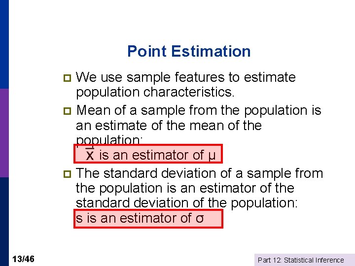
Point Estimation We use sample features to estimate population characteristics. p Mean of a sample from the population is an estimate of the mean of the population: is an estimator of μ p The standard deviation of a sample from the population is an estimator of the standard deviation of the population: s is an estimator of σ p 13/46 Part 12: Statistical Inference

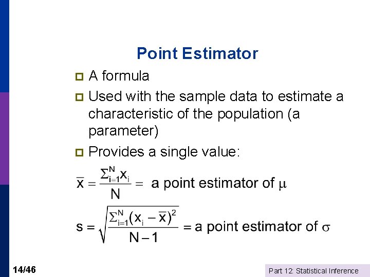
Point Estimator A formula p Used with the sample data to estimate a characteristic of the population (a parameter) p Provides a single value: p 14/46 Part 12: Statistical Inference

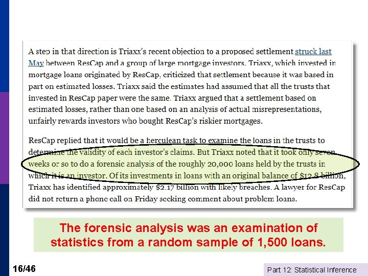
Use random samples and basic descriptive statistics. What is the ‘breach rate’ in a pool of tens of thousands of mortgages? (‘Breach’ = improperly underwritten or serviced or otherwise faulty mortgage. ) 15/46 Part 12: Statistical Inference

The forensic analysis was an examination of statistics from a random sample of 1, 500 loans. 16/46 Part 12: Statistical Inference

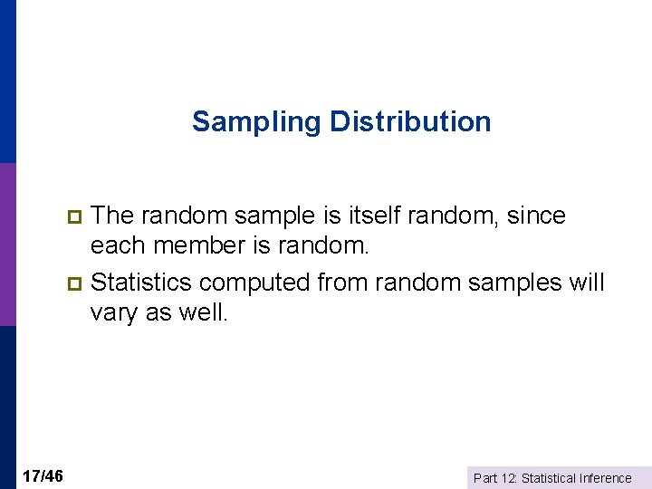
Sampling Distribution The random sample is itself random, since each member is random. p Statistics computed from random samples will vary as well. p 17/46 Part 12: Statistical Inference

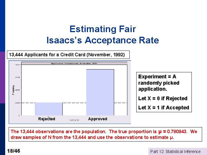
Estimating Fair Isaacs’s Acceptance Rate 13, 444 Applicants for a Credit Card (November, 1992) Experiment = A randomly picked application. Let X = 0 if Rejected Let X = 1 if Accepted Rejected Approved The 13, 444 observations are the population. The true proportion is μ = 0. 780943. We draw samples of N from the 13, 444 and use the observations to estimate μ. 18/46 Part 12: Statistical Inference

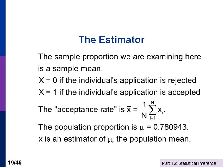
The Estimator 19/46 Part 12: Statistical Inference

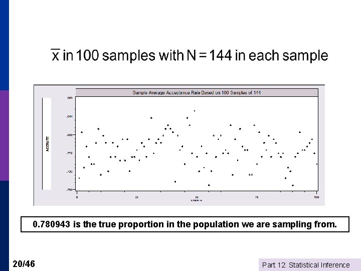
0. 780943 is the true proportion in the population we are sampling from. 20/46 Part 12: Statistical Inference

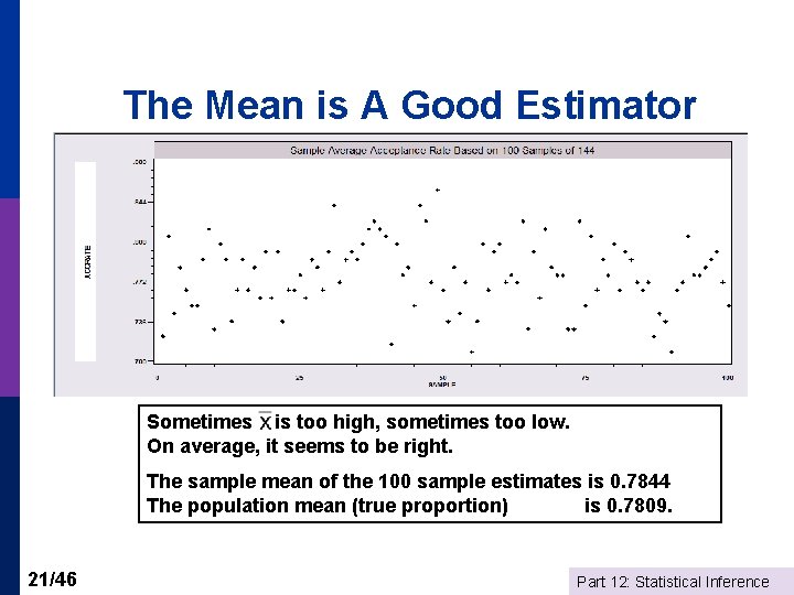
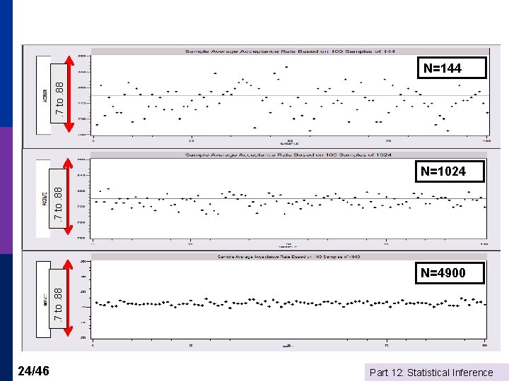
The Mean is A Good Estimator Sometimes is too high, sometimes too low. On average, it seems to be right. The sample mean of the 100 sample estimates is 0. 7844 The population mean (true proportion) is 0. 7809. 21/46 Part 12: Statistical Inference

What Makes it a Good Estimator? The average of the averages will hit the true mean (on average) p The mean is UNBIASED (No moral connotations) p 22/46 Part 12: Statistical Inference

What Does the Law of Large Numbers Say? 23/46 p The sampling variability in the estimator gets smaller as N gets larger. p If N gets large enough, we should hit the target exactly; The mean is CONSISTENT Part 12: Statistical Inference

. 7 to. 88 N=144 . 7 to. 88 N=1024 . 7 to. 88 N=4900 24/46 Part 12: Statistical Inference

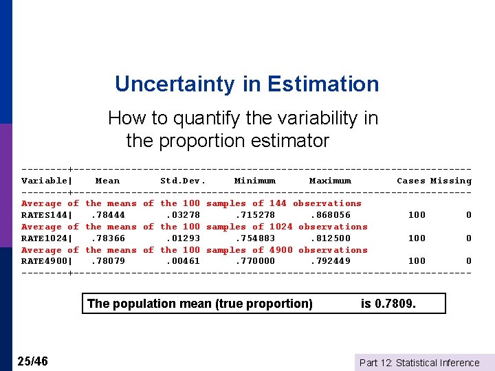
Uncertainty in Estimation How to quantify the variability in the proportion estimator ----+----------------------------------Variable| Mean Std. Dev. Minimum Maximum Cases Missing ----+----------------------------------Average of the means of the 100 samples of 144 observations RATES 144|. 78444. 03278. 715278. 868056 100 0 Average of the means of the 100 samples of 1024 observations RATE 1024|. 78366. 01293. 754883. 812500 100 0 Average of the means of the 100 samples of 4900 observations RATE 4900|. 78079. 00461. 770000. 792449 100 0 ----+----------------------------------- The population mean (true proportion) 25/46 is 0. 7809. Part 12: Statistical Inference

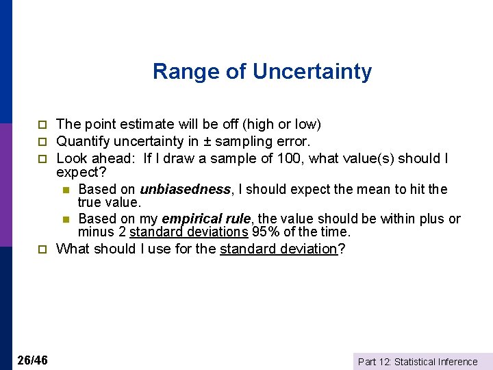
Range of Uncertainty p p 26/46 The point estimate will be off (high or low) Quantify uncertainty in ± sampling error. Look ahead: If I draw a sample of 100, what value(s) should I expect? n Based on unbiasedness, I should expect the mean to hit the true value. n Based on my empirical rule, the value should be within plus or minus 2 standard deviations 95% of the time. What should I use for the standard deviation? Part 12: Statistical Inference

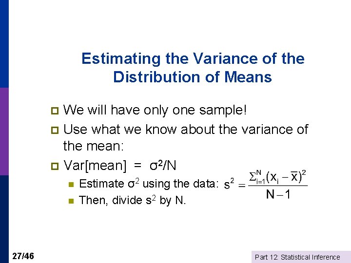
Estimating the Variance of the Distribution of Means We will have only one sample! p Use what we know about the variance of the mean: p Var[mean] = σ2/N p n n 27/46 Estimate σ2 using the data: Then, divide s 2 by N. Part 12: Statistical Inference

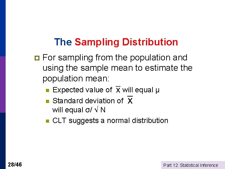
The Sampling Distribution p For sampling from the population and using the sample mean to estimate the population mean: n n n 28/46 Expected value of will equal μ Standard deviation of will equal σ/ √ N CLT suggests a normal distribution Part 12: Statistical Inference

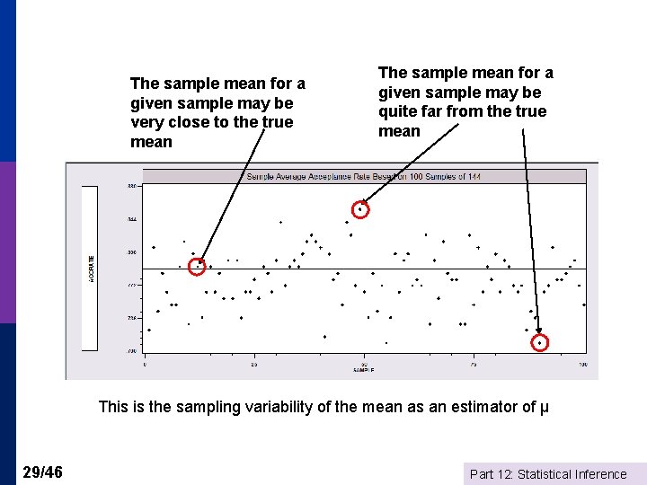
The sample mean for a given sample may be very close to the true mean The sample mean for a given sample may be quite far from the true mean This is the sampling variability of the mean as an estimator of μ 29/46 Part 12: Statistical Inference

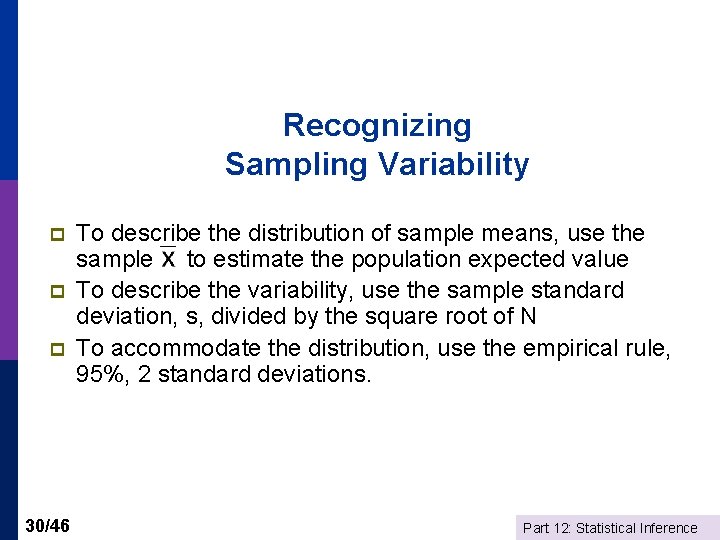
Recognizing Sampling Variability p p p 30/46 To describe the distribution of sample means, use the sample to estimate the population expected value To describe the variability, use the sample standard deviation, s, divided by the square root of N To accommodate the distribution, use the empirical rule, 95%, 2 standard deviations. Part 12: Statistical Inference

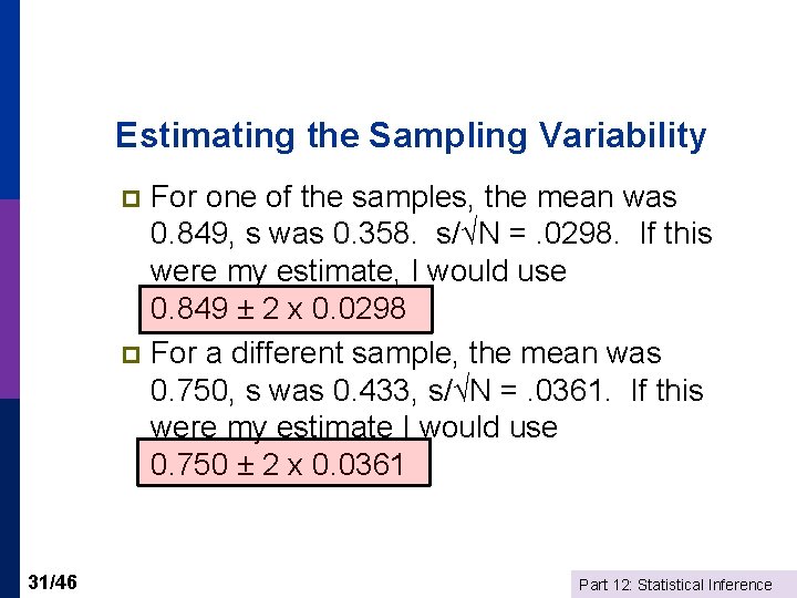
Estimating the Sampling Variability For one of the samples, the mean was 0. 849, s was 0. 358. s/√N =. 0298. If this were my estimate, I would use 0. 849 ± 2 x 0. 0298 p For a different sample, the mean was 0. 750, s was 0. 433, s/√N =. 0361. If this were my estimate I would use 0. 750 ± 2 x 0. 0361 p 31/46 Part 12: Statistical Inference

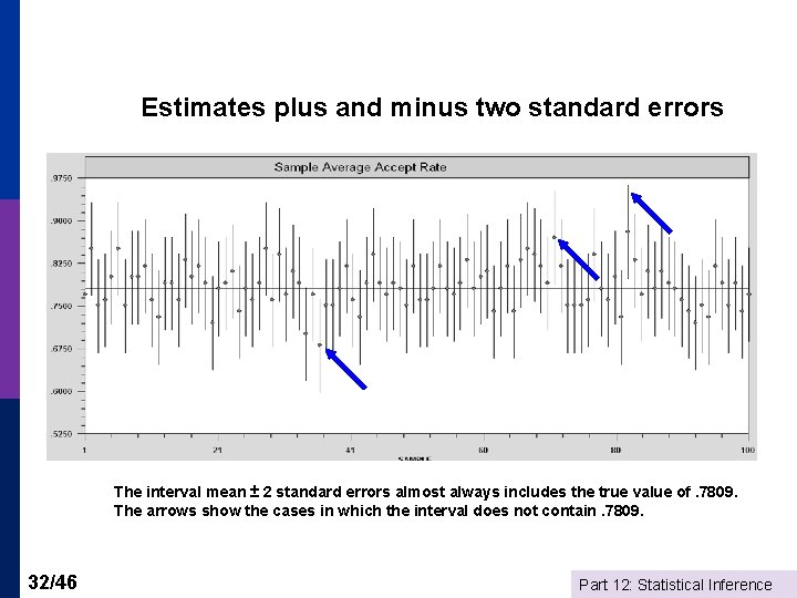
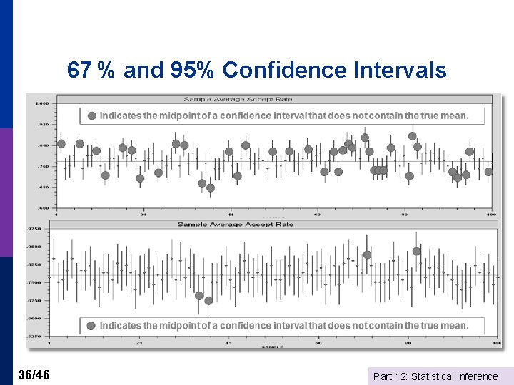
Estimates plus and minus two standard errors The interval mean ± 2 standard errors almost always includes the true value of. 7809. The arrows show the cases in which the interval does not contain. 7809. 32/46 Part 12: Statistical Inference

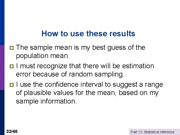
How to use these results The sample mean is my best guess of the population mean. p I must recognize that there will be estimation error because of random sampling. p I use the confidence interval to suggest a range of plausible values for the mean, based on my sample information. p 33/46 Part 12: Statistical Inference

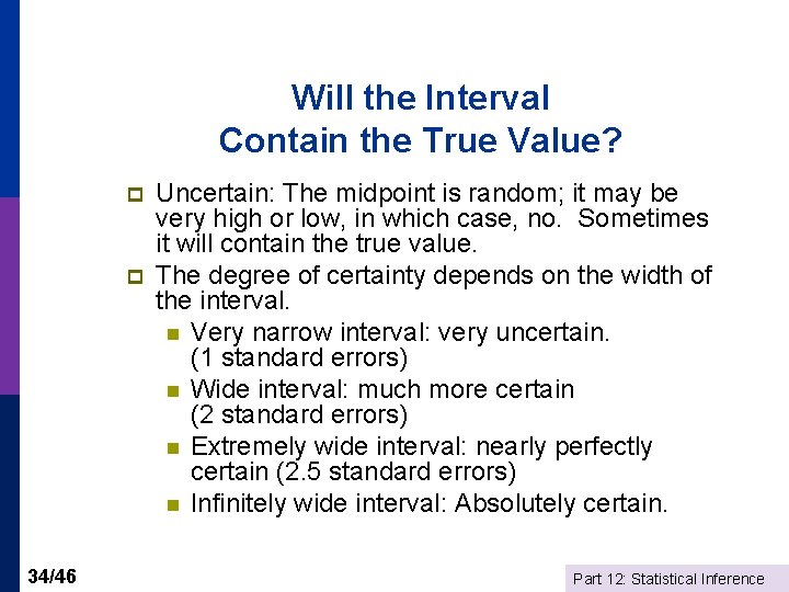
Will the Interval Contain the True Value? p p 34/46 Uncertain: The midpoint is random; it may be very high or low, in which case, no. Sometimes it will contain the true value. The degree of certainty depends on the width of the interval. n Very narrow interval: very uncertain. (1 standard errors) n Wide interval: much more certain (2 standard errors) n Extremely wide interval: nearly perfectly certain (2. 5 standard errors) n Infinitely wide interval: Absolutely certain. Part 12: Statistical Inference

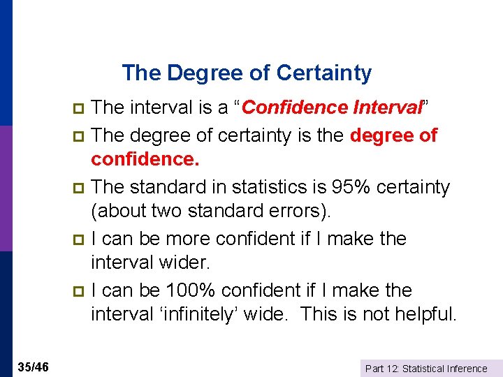
The Degree of Certainty The interval is a “Confidence Interval” p The degree of certainty is the degree of confidence. p The standard in statistics is 95% certainty (about two standard errors). p I can be more confident if I make the interval wider. p I can be 100% confident if I make the interval ‘infinitely’ wide. This is not helpful. p 35/46 Part 12: Statistical Inference

67 % and 95% Confidence Intervals 36/46 Part 12: Statistical Inference

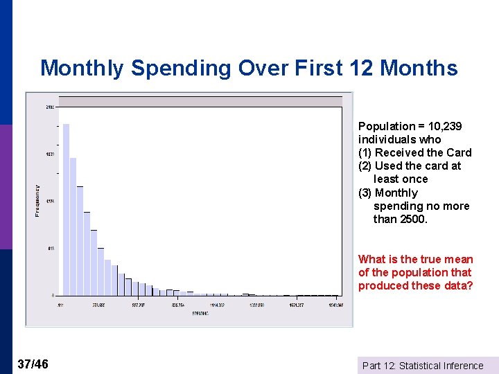
Monthly Spending Over First 12 Months Population = 10, 239 individuals who (1) Received the Card (2) Used the card at least once (3) Monthly spending no more than 2500. What is the true mean of the population that produced these data? 37/46 Part 12: Statistical Inference

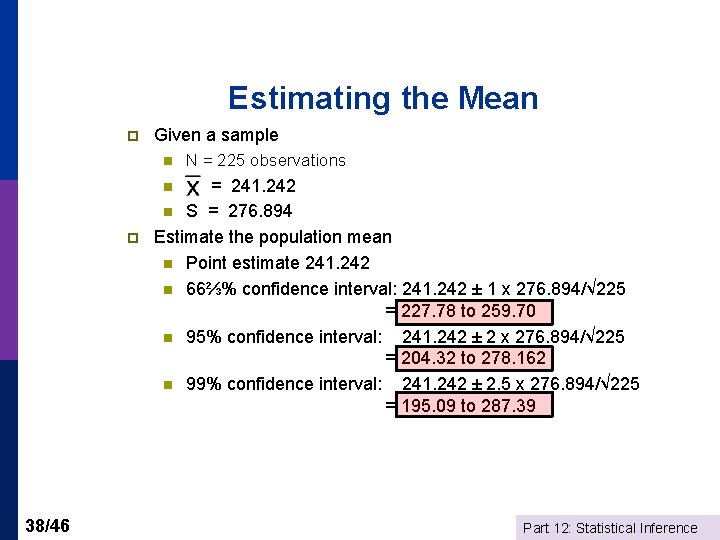
Estimating the Mean p Given a sample n N = 225 observations = 241. 242 n S = 276. 894 Estimate the population mean n Point estimate 241. 242 n 66⅔% confidence interval: 241. 242 ± 1 x 276. 894/√ 225 = 227. 78 to 259. 70 n 95% confidence interval: 241. 242 ± 2 x 276. 894/√ 225 = 204. 32 to 278. 162 n 99% confidence interval: 241. 242 ± 2. 5 x 276. 894/√ 225 = 195. 09 to 287. 39 n p 38/46 Part 12: Statistical Inference

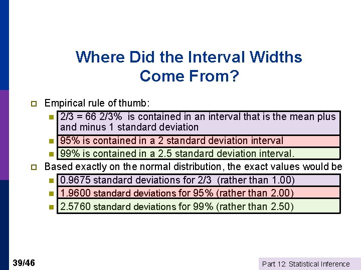
Where Did the Interval Widths Come From? p p 39/46 Empirical rule of thumb: n 2/3 = 66 2/3% is contained in an interval that is the mean plus and minus 1 standard deviation n 95% is contained in a 2 standard deviation interval n 99% is contained in a 2. 5 standard deviation interval. Based exactly on the normal distribution, the exact values would be n 0. 9675 standard deviations for 2/3 (rather than 1. 00) n 1. 9600 standard deviations for 95% (rather than 2. 00) n 2. 5760 standard deviations for 99% (rather than 2. 50) Part 12: Statistical Inference

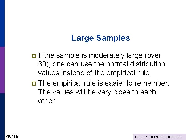
Large Samples If the sample is moderately large (over 30), one can use the normal distribution values instead of the empirical rule. p The empirical rule is easier to remember. The values will be very close to each other. p 40/46 Part 12: Statistical Inference

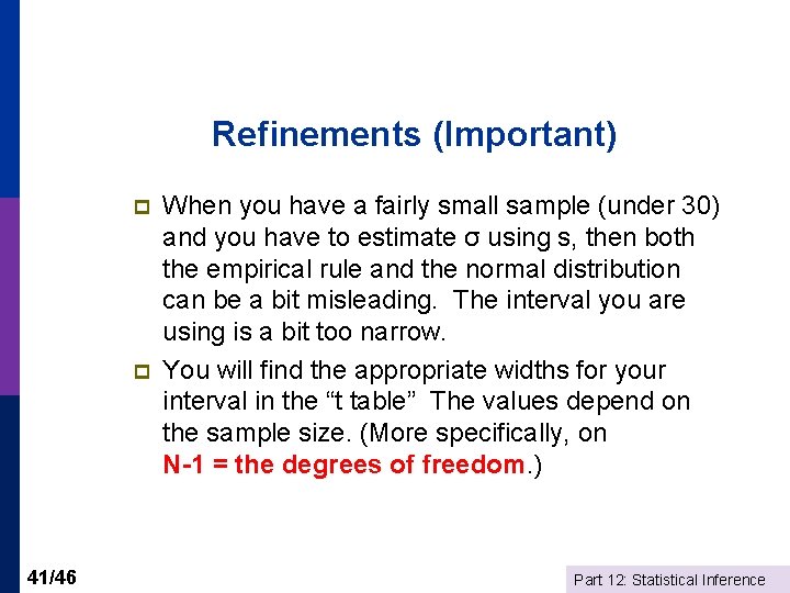
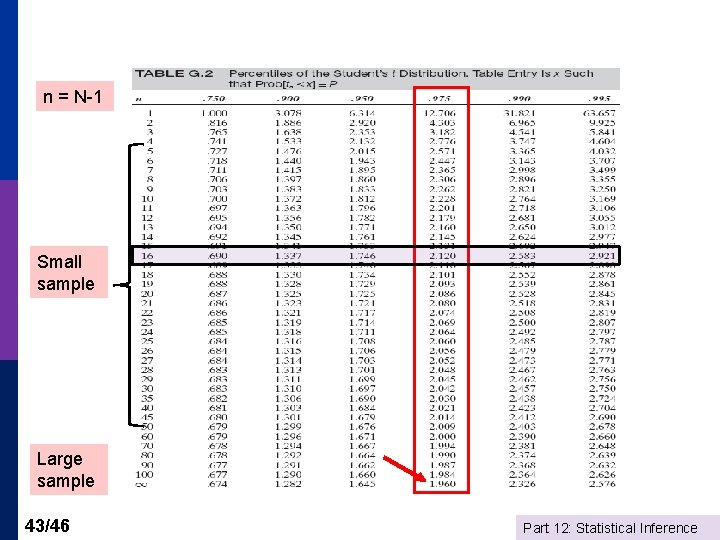
Refinements (Important) p p 41/46 When you have a fairly small sample (under 30) and you have to estimate σ using s, then both the empirical rule and the normal distribution can be a bit misleading. The interval you are using is a bit too narrow. You will find the appropriate widths for your interval in the “t table” The values depend on the sample size. (More specifically, on N-1 = the degrees of freedom. ) Part 12: Statistical Inference

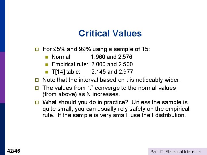
Critical Values p p 42/46 For 95% and 99% using a sample of 15: n Normal: 1. 960 and 2. 576 n Empirical rule: 2. 000 and 2. 500 n T[14] table: 2. 145 and 2. 977 Note that the interval based on t is noticeably wider. The values from “t” converge to the normal values (from above) as N increases. What should you do in practice? Unless the sample is quite small, you can usually rely safely on the empirical rule. If the sample is very small, use the t distribution. Part 12: Statistical Inference

n = N-1 Small sample Large sample 43/46 Part 12: Statistical Inference

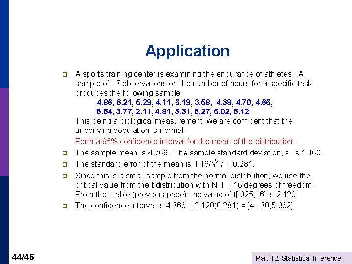
Application p p p 44/46 A sports training center is examining the endurance of athletes. A sample of 17 observations on the number of hours for a specific task produces the following sample: 4. 86, 6. 21, 5. 29, 4. 11, 6. 19, 3. 58, 4. 38, 4. 70, 4. 66, 5. 64, 3. 77, 2. 11, 4. 81, 3. 31, 6. 27, 5. 02, 6. 12 This being a biological measurement, we are confident that the underlying population is normal. Form a 95% confidence interval for the mean of the distribution. The sample mean is 4. 766. The sample standard deviation, s, is 1. 160. The standard error of the mean is 1. 16/√ 17 = 0. 281. Since this is a small sample from the normal distribution, we use the critical value from the t distribution with N-1 = 16 degrees of freedom. From the t table (previous page), the value of t[. 025, 16] is 2. 120 The confidence interval is 4. 766 ± 2. 120(0. 281) = [4. 170, 5. 362] Part 12: Statistical Inference

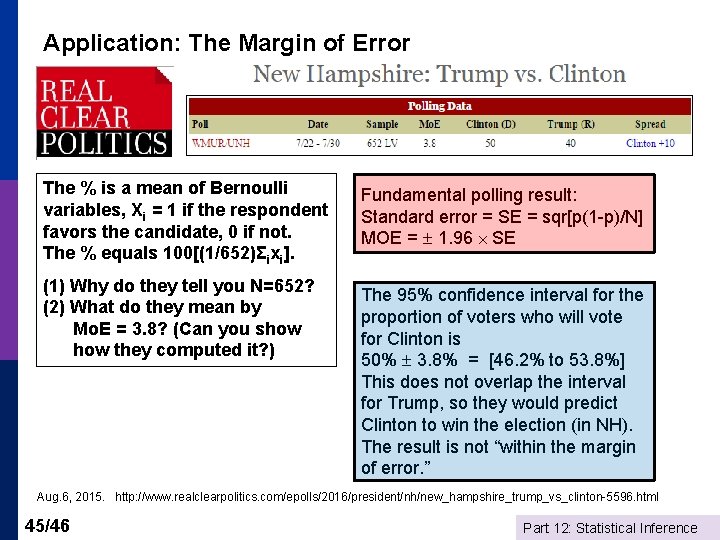
Application: The Margin of Error The % is a mean of Bernoulli variables, Xi = 1 if the respondent favors the candidate, 0 if not. The % equals 100[(1/652)Σixi]. (1) Why do they tell you N=652? (2) What do they mean by Mo. E = 3. 8? (Can you show they computed it? ) Fundamental polling result: Standard error = SE = sqr[p(1 -p)/N] MOE = 1. 96 SE The 95% confidence interval for the proportion of voters who will vote for Clinton is 50% 3. 8% = [46. 2% to 53. 8%] This does not overlap the interval for Trump, so they would predict Clinton to win the election (in NH). The result is not “within the margin of error. ” Aug. 6, 2015. http: //www. realclearpolitics. com/epolls/2016/president/nh/new_hampshire_trump_vs_clinton-5596. html 45/46 Part 12: Statistical Inference

Summary p p Methodology: Statistical Inference Application to credit scoring Sample statistics as estimators Point estimation n p p Sampling distributions Confidence intervals n n p 46/46 Sampling variability The law of large numbers Unbiasedness and consistency Proportion Mean Using the normal and t distributions instead of the empirical rule for the width of the interval. Part 12: Statistical Inference