Statistics and Data Analysis Professor William Greene Stern

Statistics and Data Analysis Professor William Greene Stern School of Business IOMS Department of Economics 1/47 Part 9: Normal Distribution

Statistics and Data Analysis Part 9 – The Normal Distribution 2/47 Part 9: Normal Distribution

The Normal Distribution p p Continuous Distributions are models n Application – The Exponential Model n Computing Probabilities for Continuous Variables Normal Distribution Model n n p 3/47 Normal Probabilities Reading the Normal Table and Computing Probabilities Applications Part 9: Normal Distribution

The Normal Distribution p p p 4/47 The most useful distribution in all branches of statistics and econometrics. Strikingly accurate model for elements of human behavior and interaction Strikingly accurate model for any random outcome that comes about as a sum of small influences. Part 9: Normal Distribution

Applications p p 5/47 Biological measurements of all sorts (not just human mental and physical) Accumulated errors in experiments Numbers of events accumulated in time n Amount of rainfall per interval n Number of stock orders per (longer) interval. (We used the Poisson for short intervals) n Economic aggregates of small terms. And on and on…. . Part 9: Normal Distribution

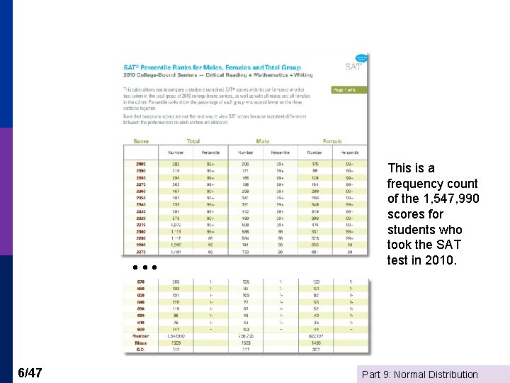
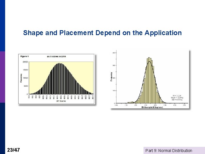
6/47 This is a frequency count of the 1, 547, 990 scores for students who took the SAT test in 2010. Part 9: Normal Distribution

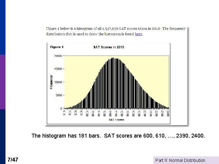
The histogram has 181 bars. SAT scores are 600, 610, …, 2390, 2400. 7/47 Part 9: Normal Distribution

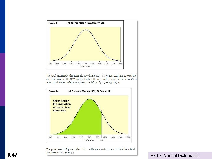
8/47 Part 9: Normal Distribution

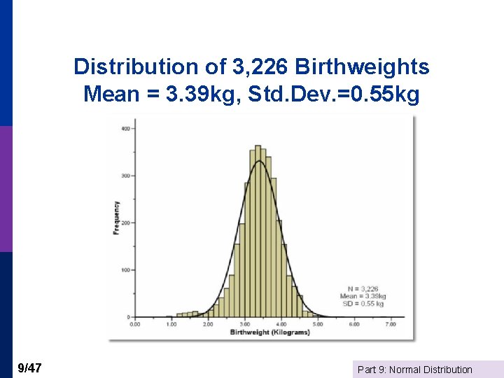
Distribution of 3, 226 Birthweights Mean = 3. 39 kg, Std. Dev. =0. 55 kg 9/47 Part 9: Normal Distribution

Continuous Distributions p p p 10/47 Continuous distributions are models for probabilities of events associated with measurements rather than counts. Continuous distributions do not occur in nature the way that discrete counting rules (e. g. , binomial) do. The random variable is a measurement, X The device is a probability density function, f(x). Probabilities are computed using calculus (and computers) Part 9: Normal Distribution

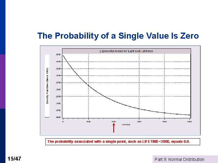
Application: Light Bulb Lifetimes p p 11/47 A box of light bulbs states “Average life is 1500 hours” P[Fails at exactly 1500 hours] is 0. 0. Note, this is exactly 1500. 00000…, not 1500. 000001, … P[Fails in an interval (1000 to 2000)] is provided by the model (as we now develop). The model being used is called the exponential model Part 9: Normal Distribution

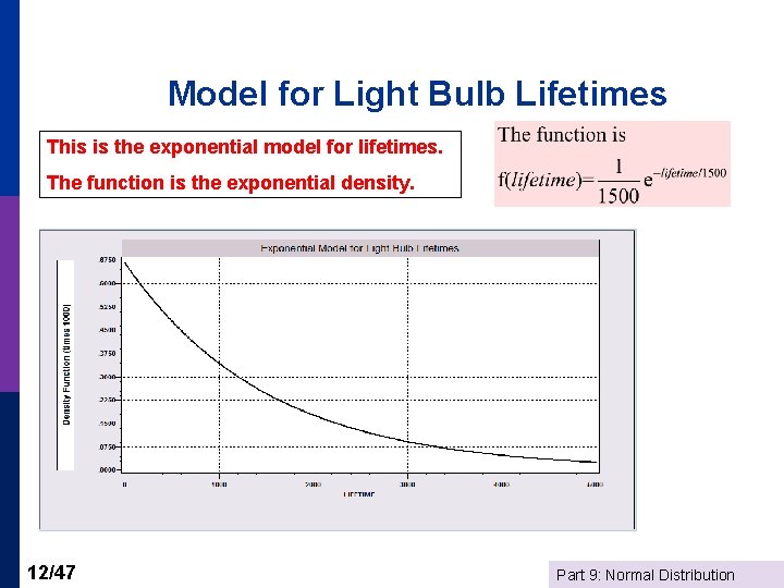
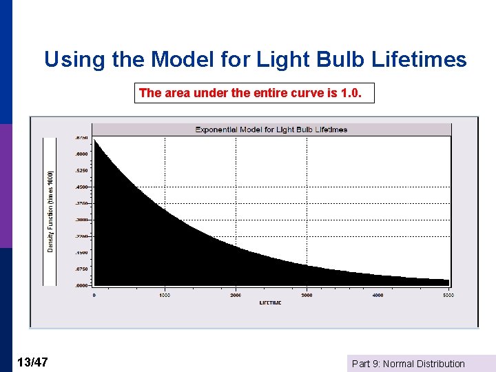
Model for Light Bulb Lifetimes This is the exponential model for lifetimes. The function is the exponential density. 12/47 Part 9: Normal Distribution

Using the Model for Light Bulb Lifetimes The area under the entire curve is 1. 0. 13/47 Part 9: Normal Distribution

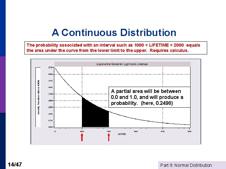
A Continuous Distribution The probability associated with an interval such as 1000 < LIFETIME < 2000 equals the area under the curve from the lower limit to the upper. Requires calculus. A partial area will be between 0. 0 and 1. 0, and will produce a probability. (here, 0. 2498) 14/47 Part 9: Normal Distribution

The Probability of a Single Value Is Zero The probability associated with a single point, such as LIFETIME=2000, equals 0. 0. 15/47 Part 9: Normal Distribution

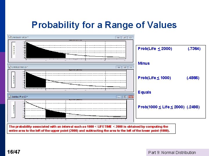
Probability for a Range of Values Prob(Life < 2000) (. 7364) Minus Prob(Life < 1000) (. 4866) Equals Prob(1000 < Life < 2000) (. 2498) The probability associated with an interval such as 1000 < LIFETIME < 2000 is obtained by computing the entire area to the left of the upper point (2000) and subtracting the area to the left of the lower point (1000). 16/47 Part 9: Normal Distribution

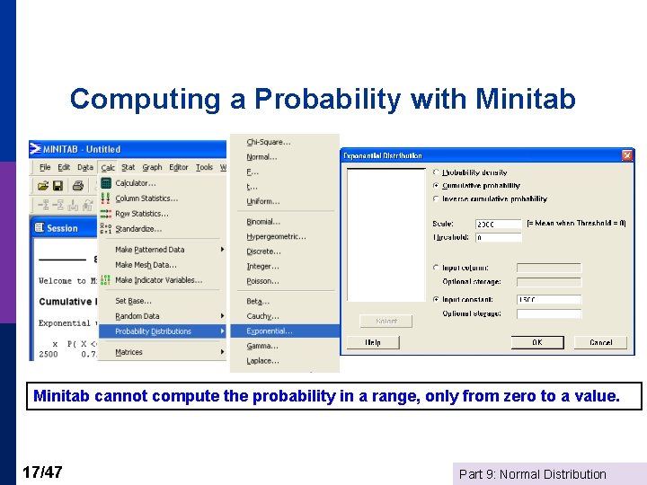
Computing a Probability with Minitab cannot compute the probability in a range, only from zero to a value. 17/47 Part 9: Normal Distribution

Applications of the Exponential Model n n n 18/47 Time between signals arriving at a switch (telephone, message center, email server, paging switch…) (This is called the “interarrival time. ”) Length of survival of transplant patients. (Survival time) Lengths of spells of unemployment Time until failure of electronic components Time until consumers use a product warranty Lifetimes of light bulbs Part 9: Normal Distribution

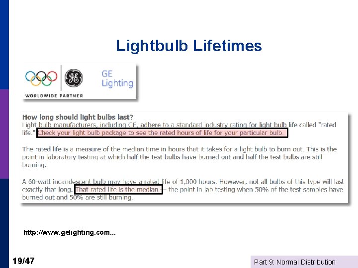
Lightbulb Lifetimes http: //www. gelighting. com. . . 19/47 Part 9: Normal Distribution

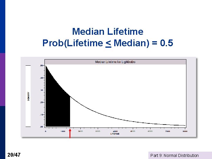
Median Lifetime Prob(Lifetime < Median) = 0. 5 20/47 Part 9: Normal Distribution

The Normal Distribution p p p 21/47 Normal Distribution Model Normal Probabilities Reading the Normal Table Computing Normal Probabilities Applications Part 9: Normal Distribution

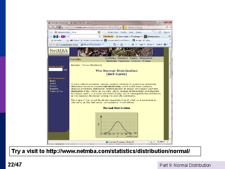
Try a visit to http: //www. netmba. com/statistics/distribution/normal/ 22/47 Part 9: Normal Distribution

Shape and Placement Depend on the Application 23/47 Part 9: Normal Distribution

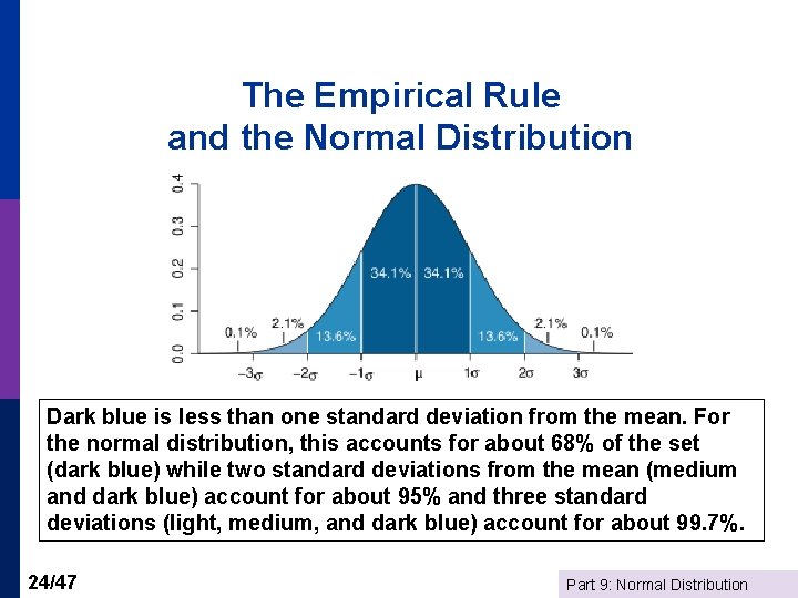
The Empirical Rule and the Normal Distribution Dark blue is less than one standard deviation from the mean. For the normal distribution, this accounts for about 68% of the set (dark blue) while two standard deviations from the mean (medium and dark blue) account for about 95% and three standard deviations (light, medium, and dark blue) account for about 99. 7%. 24/47 Part 9: Normal Distribution

Computing Probabilities P[X = a specific value] = 0. (Always) p P[a < X < b] = P[X < b] – P[X < a] p (Note, for continuous distributions, < and < are the same because of the first point above. ) p 25/47 Part 9: Normal Distribution

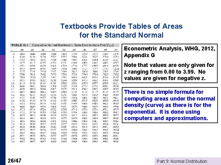
Textbooks Provide Tables of Areas for the Standard Normal Econometric Analysis, WHG, 2012, Appendix G Note that values are only given for z ranging from 0. 00 to 3. 99. No values are given for negative z. There is no simple formula for computing areas under the normal density (curve) as there is for the exponential. It is done using computers and approximations. 26/47 Part 9: Normal Distribution

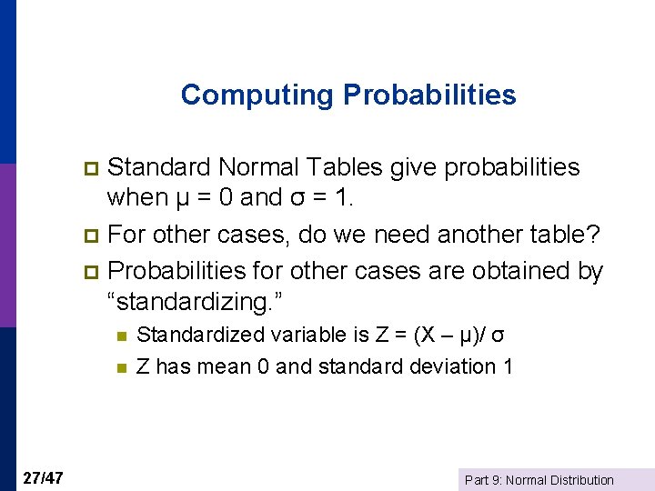
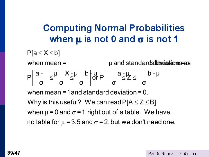
Computing Probabilities Standard Normal Tables give probabilities when μ = 0 and σ = 1. p For other cases, do we need another table? p Probabilities for other cases are obtained by “standardizing. ” p n n 27/47 Standardized variable is Z = (X – μ)/ σ Z has mean 0 and standard deviation 1 Part 9: Normal Distribution

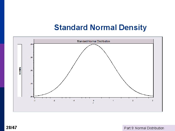
Standard Normal Density 28/47 Part 9: Normal Distribution

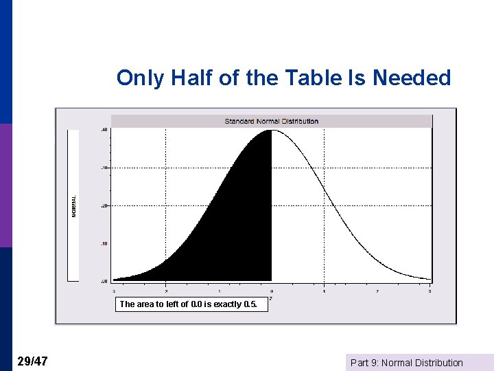
Only Half of the Table Is Needed The area to left of 0. 0 is exactly 0. 5. 29/47 Part 9: Normal Distribution

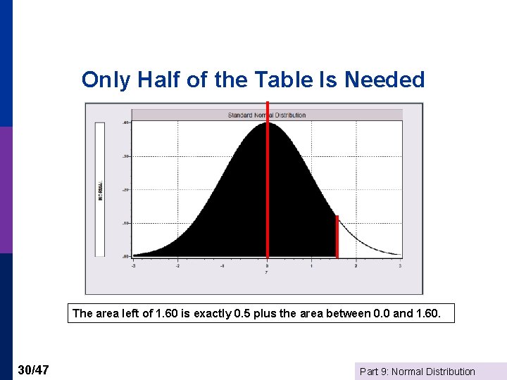
Only Half of the Table Is Needed The area left of 1. 60 is exactly 0. 5 plus the area between 0. 0 and 1. 60. 30/47 Part 9: Normal Distribution

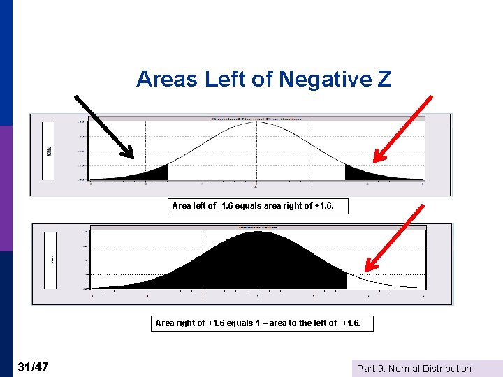
Areas Left of Negative Z Area left of -1. 6 equals area right of +1. 6. Area right of +1. 6 equals 1 – area to the left of +1. 6. 31/47 Part 9: Normal Distribution

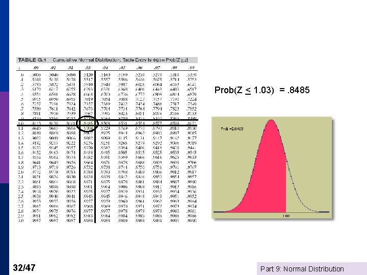
Prob(Z < 1. 03) =. 8485 32/47 Part 9: Normal Distribution

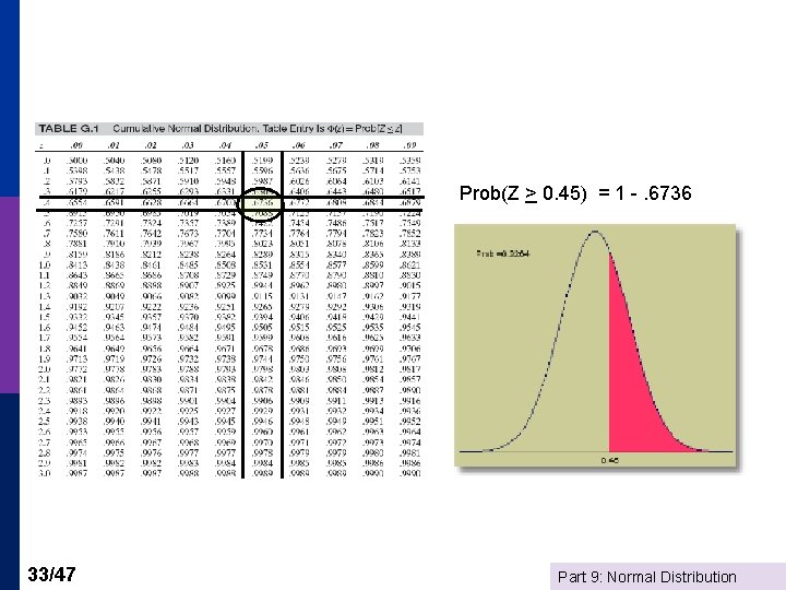
Prob(Z > 0. 45) = 1 -. 6736 33/47 Part 9: Normal Distribution

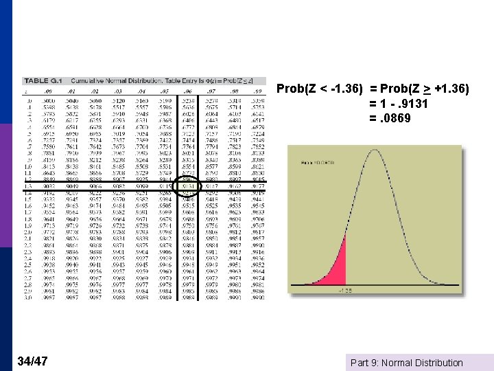
Prob(Z < -1. 36) = Prob(Z > +1. 36) = 1 -. 9131 =. 0869 34/47 Part 9: Normal Distribution

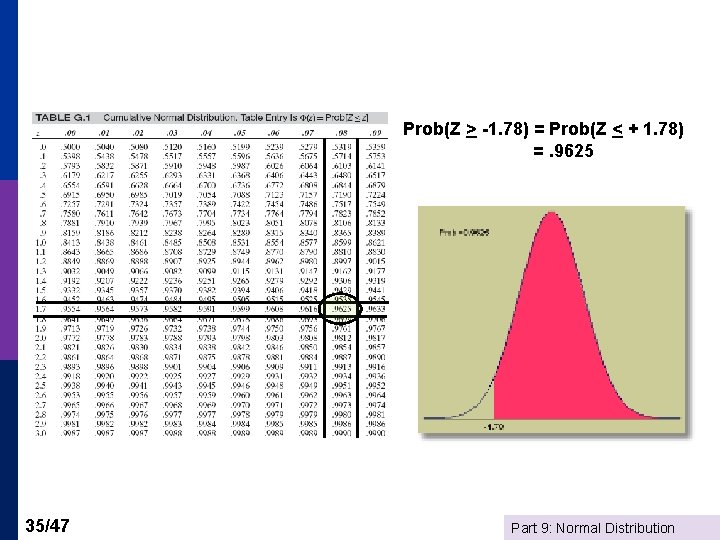
Prob(Z > -1. 78) = Prob(Z < + 1. 78) =. 9625 35/47 Part 9: Normal Distribution

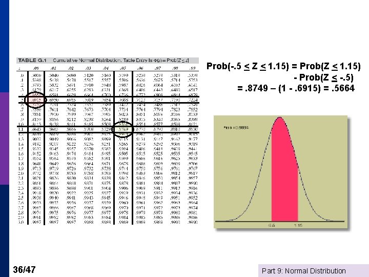
Prob(-. 5 < Z < 1. 15) = Prob(Z < 1. 15) - Prob(Z < -. 5) =. 8749 – (1 -. 6915) =. 5664 36/47 Part 9: Normal Distribution

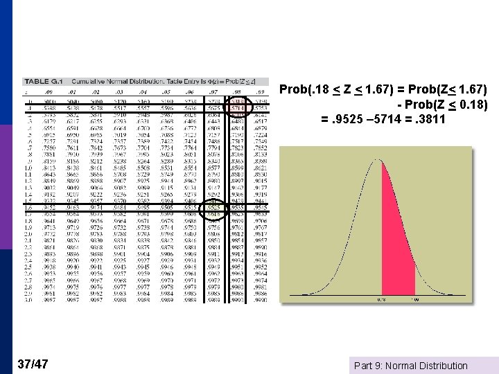
Prob(. 18 < Z < 1. 67) = Prob(Z< 1. 67) - Prob(Z < 0. 18) =. 9525 – 5714 =. 3811 37/47 Part 9: Normal Distribution

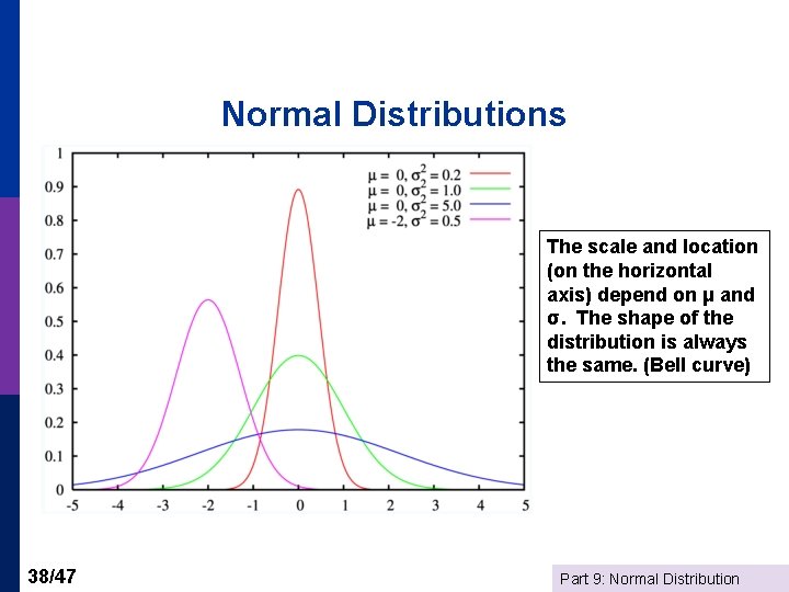
Normal Distributions The scale and location (on the horizontal axis) depend on μ and σ. The shape of the distribution is always the same. (Bell curve) 38/47 Part 9: Normal Distribution

Computing Normal Probabilities when is not 0 and is not 1 39/47 Part 9: Normal Distribution

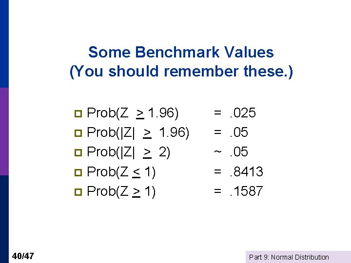
Some Benchmark Values (You should remember these. ) Prob(Z > 1. 96) p Prob(|Z| > 2) p Prob(Z < 1) p Prob(Z > 1) p 40/47 = = ~ = = . 025. 05. 8413. 1587 Part 9: Normal Distribution

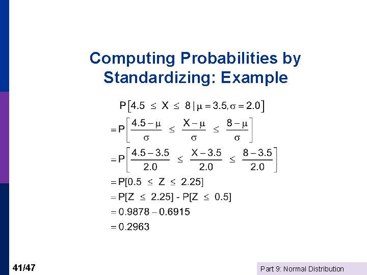
Computing Probabilities by Standardizing: Example 41/47 Part 9: Normal Distribution

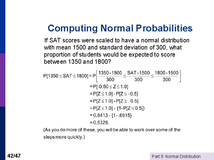
Computing Normal Probabilities If SAT scores were scaled to have a normal distribution with mean 1500 and standard deviation of 300, what proportion of students would be expected to score between 1350 and 1800? 42/47 Part 9: Normal Distribution

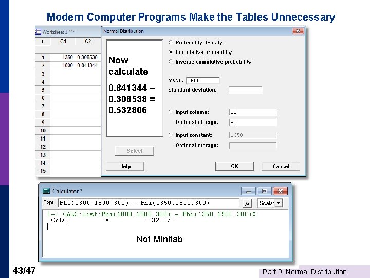
Modern Computer Programs Make the Tables Unnecessary Now calculate 0. 841344 – 0. 308538 = 0. 532806 Not Minitab 43/47 Part 9: Normal Distribution

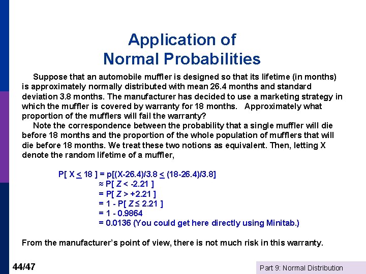
Application of Normal Probabilities Suppose that an automobile muffler is designed so that its lifetime (in months) is approximately normally distributed with mean 26. 4 months and standard deviation 3. 8 months. The manufacturer has decided to use a marketing strategy in which the muffler is covered by warranty for 18 months. Approximately what proportion of the mufflers will fail the warranty? Note the correspondence between the probability that a single muffler will die before 18 months and the proportion of the whole population of mufflers that will die before 18 months. We treat these two notions as equivalent. Then, letting X denote the random lifetime of a muffler, P[ X < 18 ] = p[(X-26. 4)/3. 8 < (18 -26. 4)/3. 8] ≈ P[ Z < -2. 21 ] = P[ Z > +2. 21 ] = 1 - P[ Z ≤ 2. 21 ] = 1 - 0. 9864 = 0. 0136 (You could get here directly using Minitab. ) From the manufacturer’s point of view, there is not much risk in this warranty. 44/47 Part 9: Normal Distribution

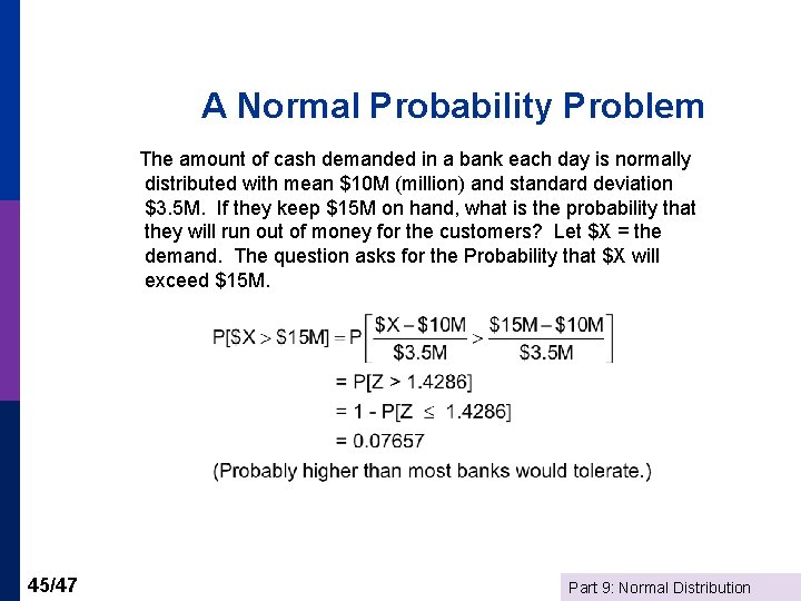
A Normal Probability Problem The amount of cash demanded in a bank each day is normally distributed with mean $10 M (million) and standard deviation $3. 5 M. If they keep $15 M on hand, what is the probability that they will run out of money for the customers? Let $X = the demand. The question asks for the Probability that $X will exceed $15 M. 45/47 Part 9: Normal Distribution

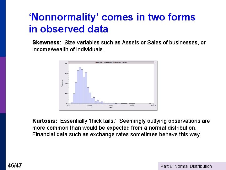
‘Nonnormality’ comes in two forms in observed data Skewness: Size variables such as Assets or Sales of businesses, or income/wealth of individuals. Kurtosis: Essentially ‘thick tails. ’ Seemingly outlying observations are more common than would be expected from a normal distribution. Financial data such as exchange rates sometimes behave this way. 46/47 Part 9: Normal Distribution

Summary p p 47/47 Continuous Distributions n Models of reality n The density function n Computing probabilities as differences of cumulative probabilities n Application to light bulb lifetimes Normal Distribution n Background n Density function depends on μ and σ n The empirical rule n Standard normal distribution n Computing normal probabilities with tables and tools Part 9: Normal Distribution