Statistics and Data Analysis Professor William Greene Stern

Statistics and Data Analysis Professor William Greene Stern School of Business IOMS Department of Economics 24 -1/45 Part 24: Multiple Regression – Part 4

Statistics and Data Analysis Part 24 – Multiple Regression: 4 24 -2/45 Part 24: Multiple Regression – Part 4

Hypothesis Tests in Multiple Regression Simple regression: Test β = 0 p Testing about individual coefficients in a multiple regression p R 2 as the fit measure in a multiple regression p n n n 24 -3/45 Testing R 2 = 0 Testing about sets of coefficients Testing whether two groups have the same model Part 24: Multiple Regression – Part 4

Regression Analysis p p p Investigate: Is the coefficient in a regression model really nonzero? Testing procedure: n Model: y = α + βx + ε n Hypothesis: H 0: β = 0. n Rejection region: Least squares coefficient is far from zero. Test: n α level for the test = 0. 05 as usual Degrees of n Compute t = b/Standard. Error Freedom for n Reject H 0 if t is above the critical value p p n 24 -4/45 the t statistic is N-2 1. 96 if large sample Value from t table if small sample. Reject H 0 if reported P value is less than α level Part 24: Multiple Regression – Part 4

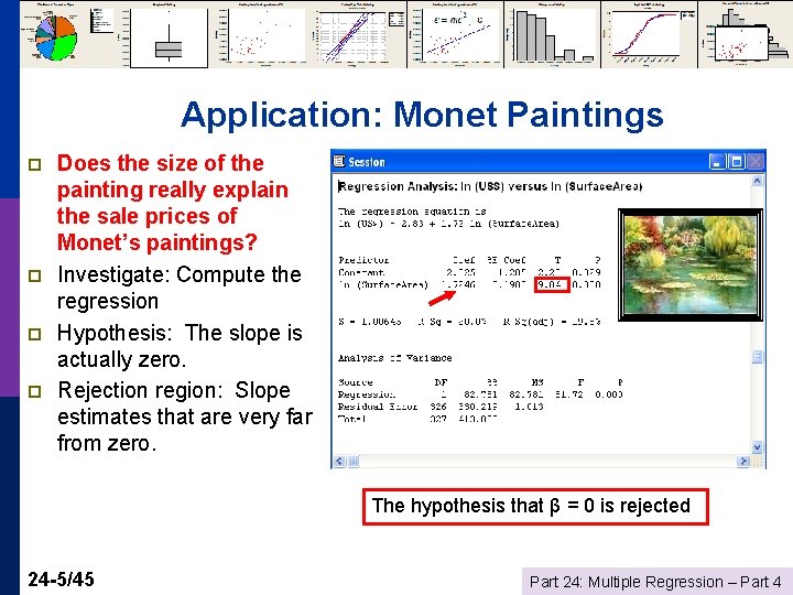
Application: Monet Paintings p p Does the size of the painting really explain the sale prices of Monet’s paintings? Investigate: Compute the regression Hypothesis: The slope is actually zero. Rejection region: Slope estimates that are very far from zero. The hypothesis that β = 0 is rejected 24 -5/45 Part 24: Multiple Regression – Part 4

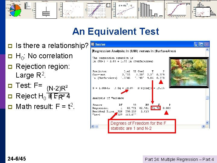
An Equivalent Test p p p Is there a relationship? H 0: No correlation Rejection region: Large R 2. Test: F= Reject H 0 if F > 4 Math result: F = t 2. Degrees of Freedom for the F statistic are 1 and N-2 24 -6/45 Part 24: Multiple Regression – Part 4

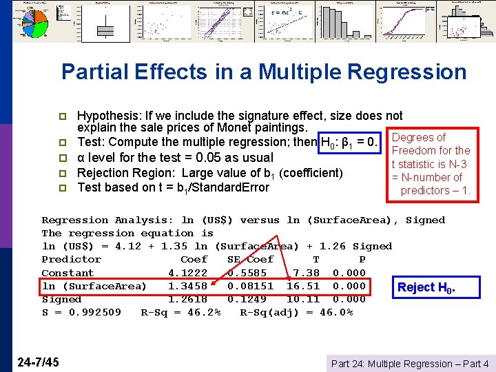
Partial Effects in a Multiple Regression p p Hypothesis: If we include the signature effect, size does not explain the sale prices of Monet paintings. Test: Compute the multiple regression; then H 0: β 1 = 0. Degrees of p α level for the test = 0. 05 as usual p Rejection Region: Large value of b 1 (coefficient) Test based on t = b 1/Standard. Error p Freedom for the t statistic is N-3 = N-number of predictors – 1. Regression Analysis: ln (US$) versus ln (Surface. Area), Signed The regression equation is ln (US$) = 4. 12 + 1. 35 ln (Surface. Area) + 1. 26 Signed Predictor Coef SE Coef T P Constant 4. 1222 0. 5585 7. 38 0. 000 ln (Surface. Area) 1. 3458 0. 08151 16. 51 0. 000 Reject H 0. Signed 1. 2618 0. 1249 10. 11 0. 000 S = 0. 992509 R-Sq = 46. 2% R-Sq(adj) = 46. 0% 24 -7/45 Part 24: Multiple Regression – Part 4

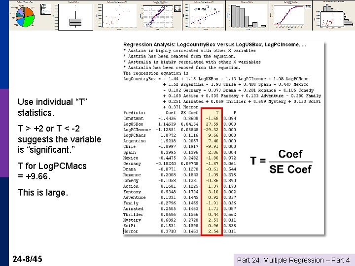
Use individual “T” statistics. T > +2 or T < -2 suggests the variable is “significant. ” T for Log. PCMacs = +9. 66. This is large. 24 -8/45 Part 24: Multiple Regression – Part 4

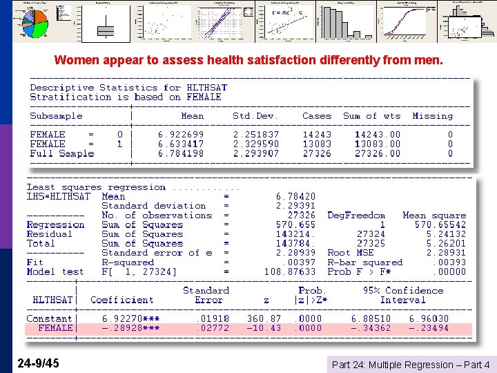
Women appear to assess health satisfaction differently from men. 24 -9/45 Part 24: Multiple Regression – Part 4

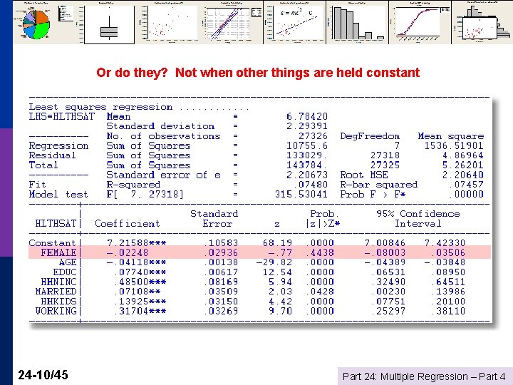
Or do they? Not when other things are held constant 24 -10/45 Part 24: Multiple Regression – Part 4

24 -11/45 Part 24: Multiple Regression – Part 4

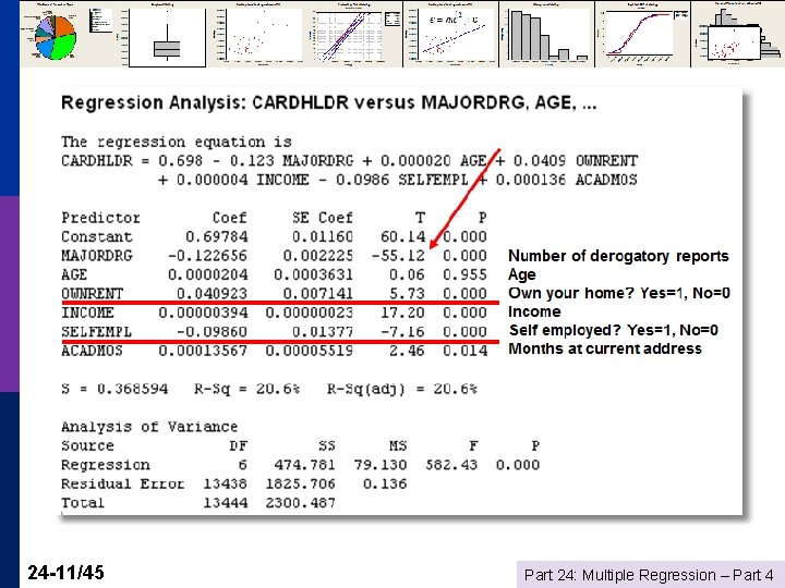
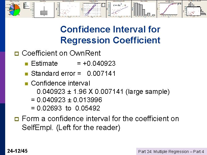
Confidence Interval for Regression Coefficient p Coefficient on Own. Rent n n n p Estimate = +0. 040923 Standard error = 0. 007141 Confidence interval 0. 040923 ± 1. 96 X 0. 007141 (large sample) = 0. 040923 ± 0. 013996 = 0. 02693 to 0. 05492 Form a confidence interval for the coefficient on Self. Empl. (Left for the reader) 24 -12/45 Part 24: Multiple Regression – Part 4

Model Fit How well does the model fit the data? p R 2 measures fit – the larger the better p n n Time series: expect. 9 or better Cross sections: it depends Social science data: . 1 is good p Industry or market data: . 5 is routine p p 24 -13/45 Use R 2 to compare models and find the right model Part 24: Multiple Regression – Part 4

Dear Prof William I hope you are doing great. I have got one of your presentations on Statistics and Data Analysis, particularly on regression modeling. There you said that R squared value could come around. 2 and not bad for large scale survey data. Currently, I am working on a large scale survey data set data (1975 samples) and r squared value came as. 30 which is low. So, I need to justify this. I thought to consider your presentation in this case. However, do you have any reference book which I can refer while justifying low r squared value of my findings? The purpose is scientific article. 24 -14/45 Part 24: Multiple Regression – Part 4

Pretty Good Fit: R 2 =. 722 Regression of Fuel Bill on Number of Rooms 24 -15/45 Part 24: Multiple Regression – Part 4

A Huge Theorem 24 -16/45 p R 2 always goes up when you add variables to your model. p Always. Part 24: Multiple Regression – Part 4

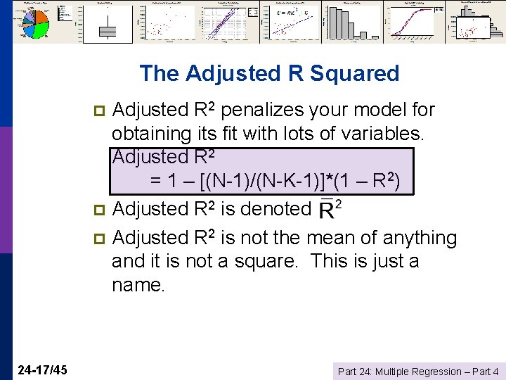
The Adjusted R Squared Adjusted R 2 penalizes your model for obtaining its fit with lots of variables. Adjusted R 2 = 1 – [(N-1)/(N-K-1)]*(1 – R 2) p Adjusted R 2 is denoted p Adjusted R 2 is not the mean of anything and it is not a square. This is just a name. p 24 -17/45 Part 24: Multiple Regression – Part 4

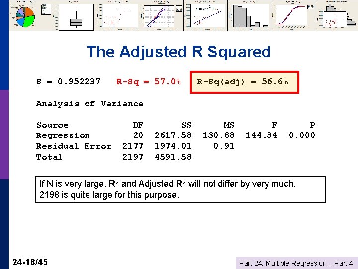
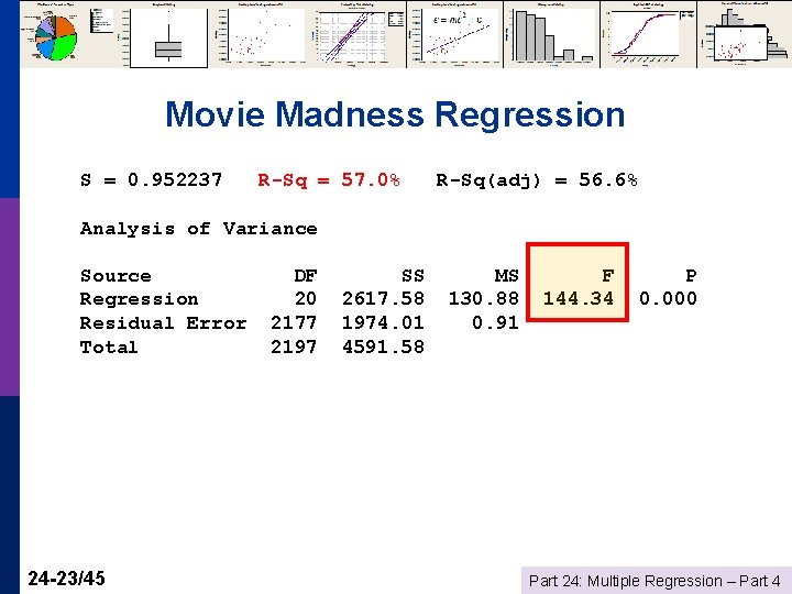
The Adjusted R Squared S = 0. 952237 R-Sq = 57. 0% R-Sq(adj) = 56. 6% Analysis of Variance Source Regression Residual Error Total DF 20 2177 2197 SS 2617. 58 1974. 01 4591. 58 MS 130. 88 0. 91 F 144. 34 P 0. 000 If N is very large, R 2 and Adjusted R 2 will not differ by very much. 2198 is quite large for this purpose. 24 -18/45 Part 24: Multiple Regression – Part 4

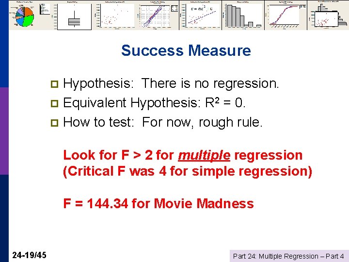
Success Measure Hypothesis: There is no regression. p Equivalent Hypothesis: R 2 = 0. p How to test: For now, rough rule. p Look for F > 2 for multiple regression (Critical F was 4 for simple regression) F = 144. 34 for Movie Madness 24 -19/45 Part 24: Multiple Regression – Part 4

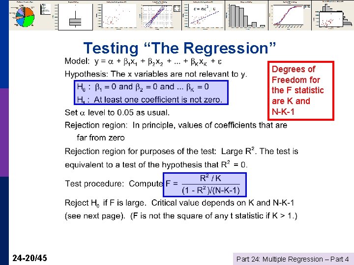
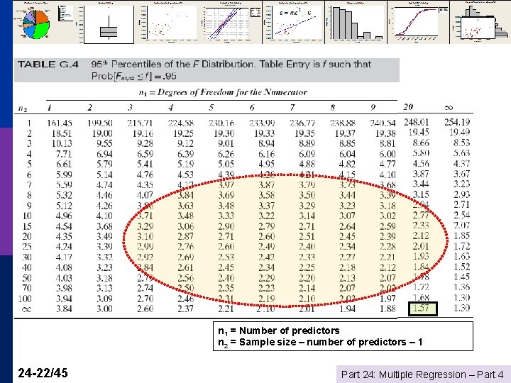
Testing “The Regression” Degrees of Freedom for the F statistic are K and N-K-1 24 -20/45 Part 24: Multiple Regression – Part 4

The F Test for the Model Determine the appropriate “critical” value from the table. p Is the F from the computed model larger than theoretical F from the table? p n n 24 -21/45 Yes: Conclude the relationship is significant No: Conclude R 2= 0. Part 24: Multiple Regression – Part 4

n 1 = Number of predictors n 2 = Sample size – number of predictors – 1 24 -22/45 Part 24: Multiple Regression – Part 4

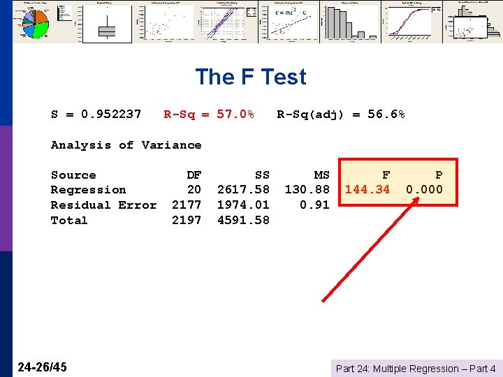
Movie Madness Regression S = 0. 952237 R-Sq = 57. 0% R-Sq(adj) = 56. 6% Analysis of Variance Source Regression Residual Error Total 24 -23/45 DF 20 2177 2197 SS 2617. 58 1974. 01 4591. 58 MS 130. 88 0. 91 F 144. 34 P 0. 000 Part 24: Multiple Regression – Part 4

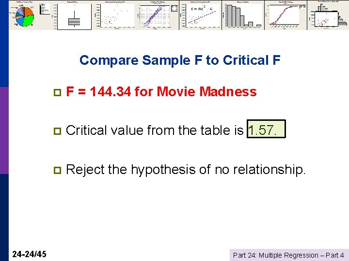
Compare Sample F to Critical F 24 -24/45 p F = 144. 34 for Movie Madness p Critical value from the table is 1. 57. p Reject the hypothesis of no relationship. Part 24: Multiple Regression – Part 4

An Equivalent Approach p p p 24 -25/45 What is the “P Value? ” We observed an F of 144. 34 (or, whatever it is). If there really were no relationship, how likely is it that we would have observed an F this large (or larger)? n Depends on N and K n The probability is reported with the regression results as the P Value. Part 24: Multiple Regression – Part 4

The F Test S = 0. 952237 R-Sq = 57. 0% R-Sq(adj) = 56. 6% Analysis of Variance Source Regression Residual Error Total 24 -26/45 DF 20 2177 2197 SS 2617. 58 1974. 01 4591. 58 MS 130. 88 0. 91 F 144. 34 P 0. 000 Part 24: Multiple Regression – Part 4

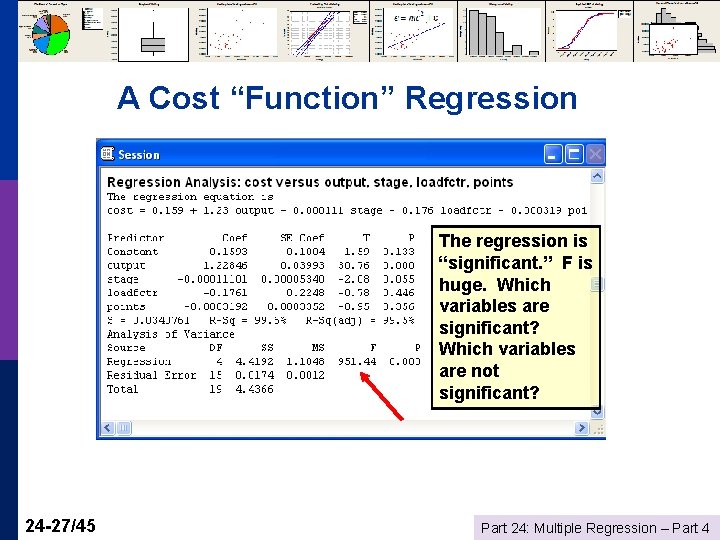
A Cost “Function” Regression The regression is “significant. ” F is huge. Which variables are significant? Which variables are not significant? 24 -27/45 Part 24: Multiple Regression – Part 4

What About a Group of Variables? p Is Genre significant in the movie model? n n n p 24 -28/45 There are 12 genre variables Some are “significant” (fantasy, mystery, horror) some are not. Can we conclude the group as a whole is? Maybe. We need a test. Part 24: Multiple Regression – Part 4

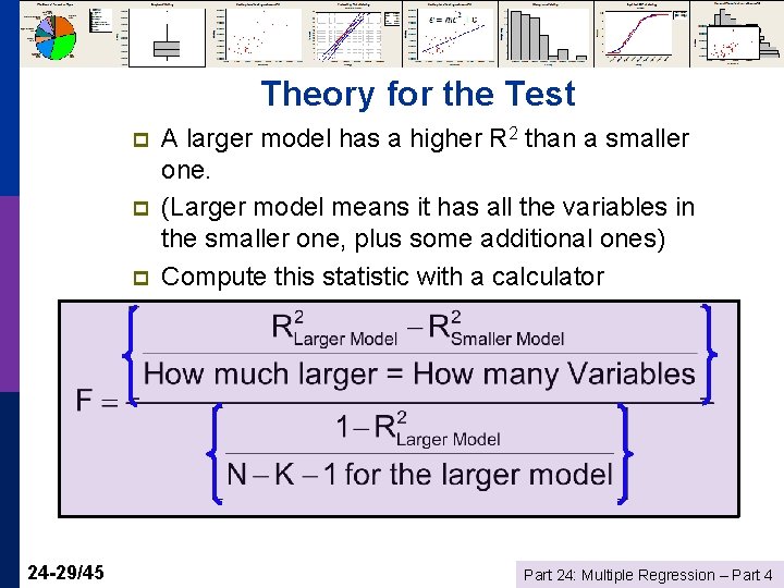
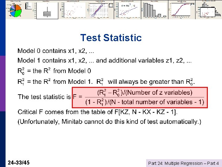
Theory for the Test p p p 24 -29/45 A larger model has a higher R 2 than a smaller one. (Larger model means it has all the variables in the smaller one, plus some additional ones) Compute this statistic with a calculator Part 24: Multiple Regression – Part 4

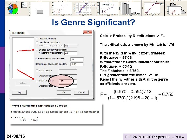
Is Genre Significant? Calc -> Probability Distributions -> F… The critical value shown by Minitab is 1. 76 With the 12 Genre indicator variables: R-Squared = 57. 0% Without the 12 Genre indicator variables: R-Squared = 55. 4% The F statistic is 6. 750. F is greater than the critical value. Reject the hypothesis that all the genre coefficients are zero. 24 -30/45 Part 24: Multiple Regression – Part 4

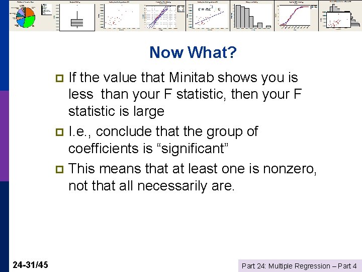
Now What? If the value that Minitab shows you is less than your F statistic, then your F statistic is large p I. e. , conclude that the group of coefficients is “significant” p This means that at least one is nonzero, not that all necessarily are. p 24 -31/45 Part 24: Multiple Regression – Part 4

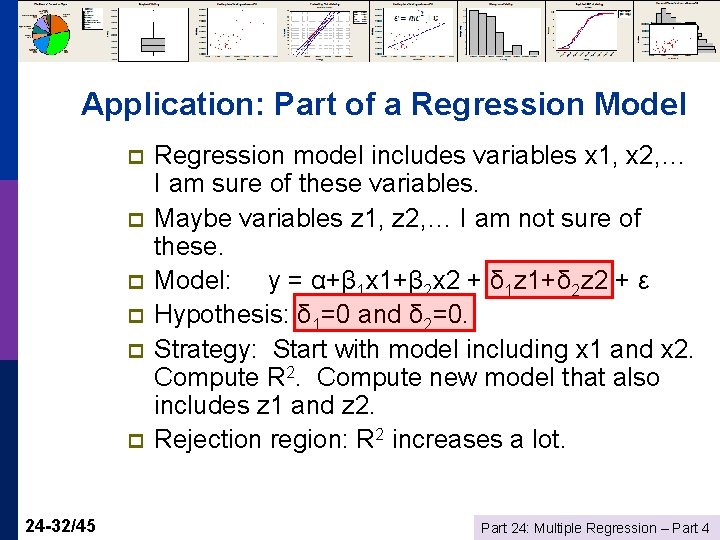
Application: Part of a Regression Model p p p 24 -32/45 Regression model includes variables x 1, x 2, … I am sure of these variables. Maybe variables z 1, z 2, … I am not sure of these. Model: y = α+β 1 x 1+β 2 x 2 + δ 1 z 1+δ 2 z 2 + ε Hypothesis: δ 1=0 and δ 2=0. Strategy: Start with model including x 1 and x 2. Compute R 2. Compute new model that also includes z 1 and z 2. Rejection region: R 2 increases a lot. Part 24: Multiple Regression – Part 4

Test Statistic 24 -33/45 Part 24: Multiple Regression – Part 4

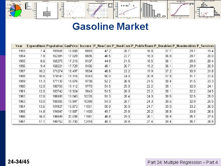
Gasoline Market 24 -34/45 Part 24: Multiple Regression – Part 4

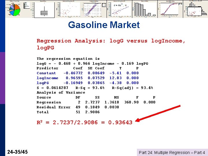
Gasoline Market Regression Analysis: log. G versus log. Income, log. PG The regression equation is log. G = - 0. 468 + 0. 966 log. Income - 0. 169 log. PG Predictor Coef SE Coef T P Constant -0. 46772 0. 08649 -5. 41 0. 000 log. Income 0. 96595 0. 07529 12. 83 0. 000 log. PG -0. 16949 0. 03865 -4. 38 0. 000 S = 0. 0614287 R-Sq = 93. 6% R-Sq(adj) = 93. 4% Analysis of Variance Source DF SS MS F P Regression 2 2. 7237 1. 3618 360. 90 0. 000 Residual Error 49 0. 1849 0. 0038 Total 51 2. 9086 R 2 = 2. 7237/2. 9086 = 0. 93643 24 -35/45 Part 24: Multiple Regression – Part 4

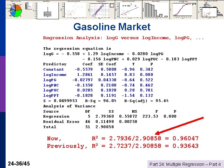
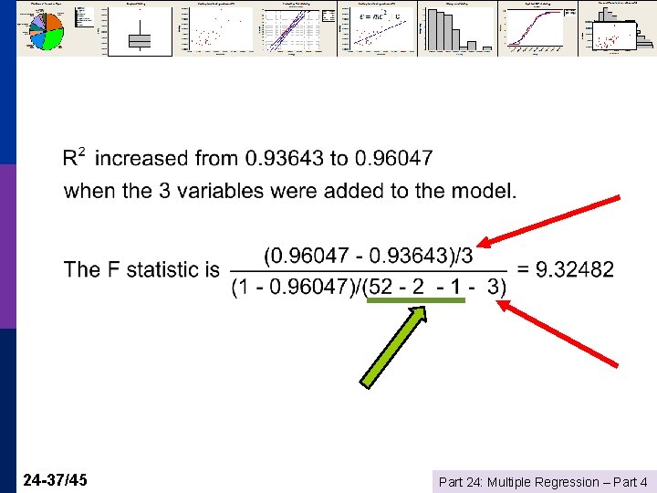
Gasoline Market Regression Analysis: log. G versus log. Income, log. PG, . . . The regression equation is log. G = - 0. 558 + 1. 29 log. Income - 0. 0280 log. PG - 0. 156 log. PNC + 0. 029 log. PUC - 0. 183 log. PPT Predictor Coef SE Coef T P Constant -0. 5579 0. 5808 -0. 96 0. 342 log. Income 1. 2861 0. 1457 8. 83 0. 000 log. PG -0. 02797 0. 04338 -0. 64 0. 522 log. PNC -0. 1558 0. 2100 -0. 74 0. 462 log. PUC 0. 0285 0. 1020 0. 28 0. 781 log. PPT -0. 1828 0. 1191 -1. 54 0. 132 S = 0. 0499953 R-Sq = 96. 0% R-Sq(adj) = 95. 6% Analysis of Variance Source DF SS MS F P Regression 5 2. 79360 0. 55872 223. 53 0. 000 Residual Error 46 0. 11498 0. 00250 Total 51 2. 90858 Now, R 2 = 2. 7936/2. 90858 = 0. 96047 Previously, R 2 = 2. 7237/2. 90858 = 0. 93643 24 -36/45 Part 24: Multiple Regression – Part 4

24 -37/45 Part 24: Multiple Regression – Part 4

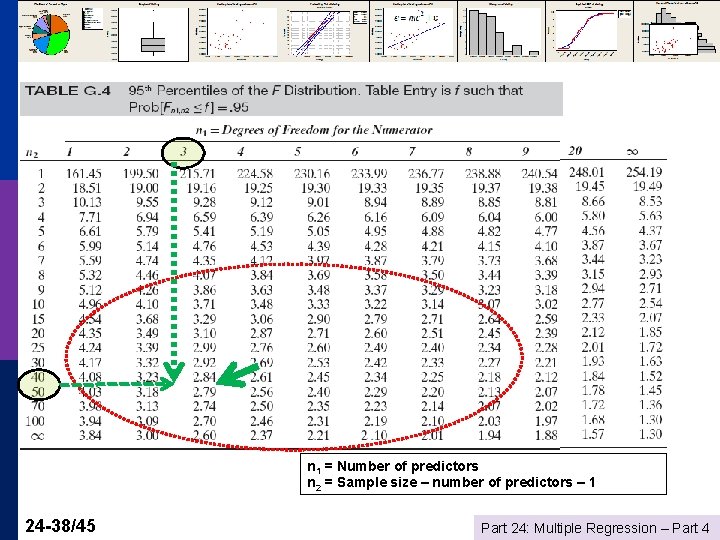
n 1 = Number of predictors n 2 = Sample size – number of predictors – 1 24 -38/45 Part 24: Multiple Regression – Part 4

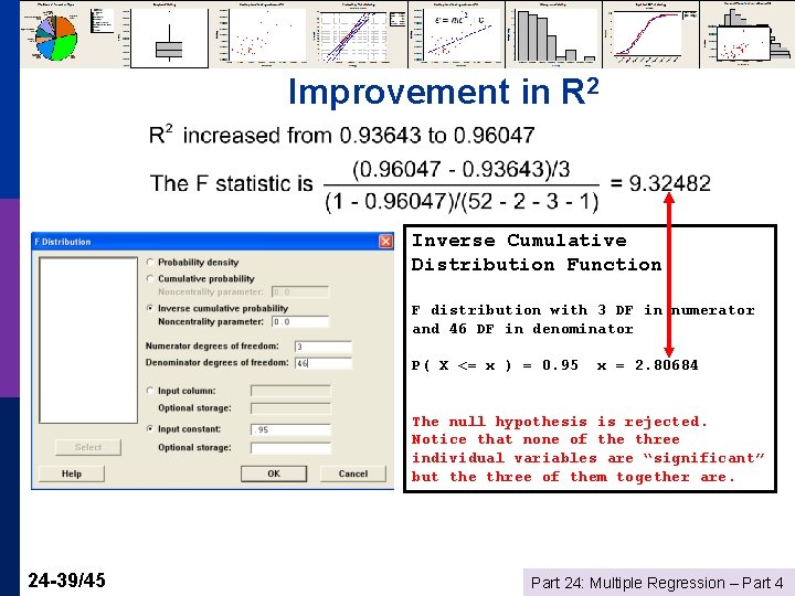
Improvement in R 2 Inverse Cumulative Distribution Function F distribution with 3 DF in numerator and 46 DF in denominator P( X <= x ) = 0. 95 x = 2. 80684 The null hypothesis is rejected. Notice that none of the three individual variables are “significant” but the three of them together are. 24 -39/45 Part 24: Multiple Regression – Part 4

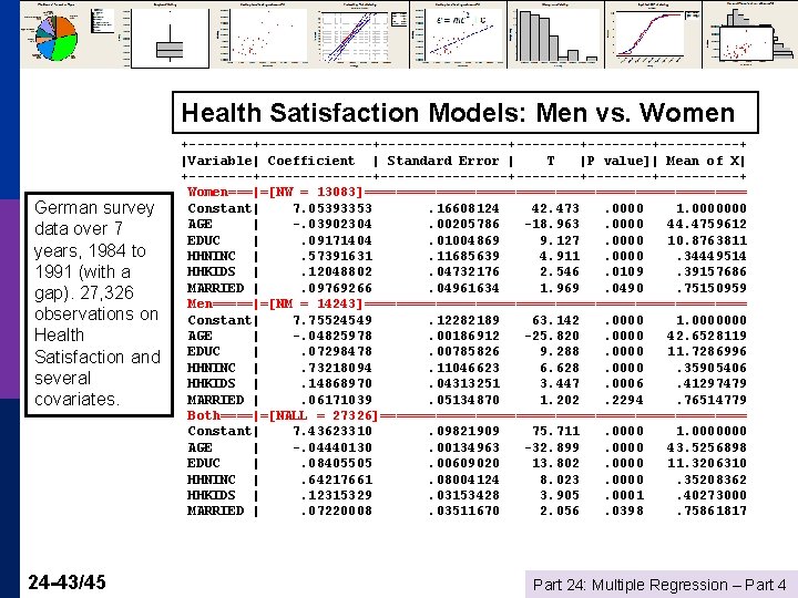
Application p Health satisfaction depends on many factors: n n p p p 24 -40/45 Age, Income, Children, Education, Marital Status Do these factors figure differently in a model for women compared to one for men? Investigation: Multiple regression Null hypothesis: The regressions are the same. Rejection Region: Estimated regressions that are very different. Part 24: Multiple Regression – Part 4

Equal Regressions Setting: Two groups of observations (men/women, countries, two different periods, firms, etc. ) p Regression Model: y = α+β 1 x 1+β 2 x 2 + … + ε p Hypothesis: The same model applies to both groups p Rejection region: Large values of F p 24 -41/45 Part 24: Multiple Regression – Part 4

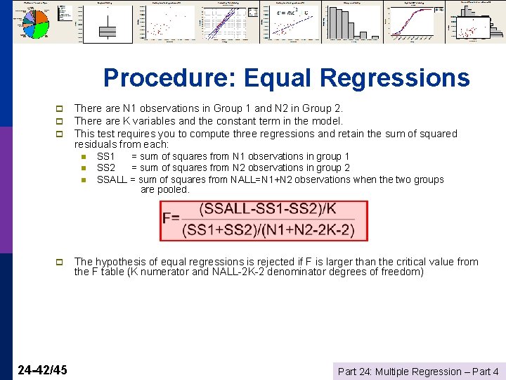
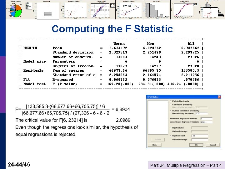
Procedure: Equal Regressions p p p There are N 1 observations in Group 1 and N 2 in Group 2. There are K variables and the constant term in the model. This test requires you to compute three regressions and retain the sum of squared residuals from each: n n n p 24 -42/45 SS 1 = sum of squares from N 1 observations in group 1 SS 2 = sum of squares from N 2 observations in group 2 SSALL = sum of squares from NALL=N 1+N 2 observations when the two groups are pooled. The hypothesis of equal regressions is rejected if F is larger than the critical value from the F table (K numerator and NALL-2 K-2 denominator degrees of freedom) Part 24: Multiple Regression – Part 4

Health Satisfaction Models: Men vs. Women German survey data over 7 years, 1984 to 1991 (with a gap). 27, 326 observations on Health Satisfaction and several covariates. 24 -43/45 +--------------+--------+--------+-----+ |Variable| Coefficient | Standard Error | T |P value]| Mean of X| +--------------+--------+--------+-----+ Women===|=[NW = 13083]======================== Constant| 7. 05393353. 16608124 42. 473. 0000 1. 0000000 AGE | -. 03902304. 00205786 -18. 963. 0000 44. 4759612 EDUC |. 09171404. 01004869 9. 127. 0000 10. 8763811 HHNINC |. 57391631. 11685639 4. 911. 0000. 34449514 HHKIDS |. 12048802. 04732176 2. 546. 0109. 39157686 MARRIED |. 09769266. 04961634 1. 969. 0490. 75150959 Men=====|=[NM = 14243]======================== Constant| 7. 75524549. 12282189 63. 142. 0000 1. 0000000 AGE | -. 04825978. 00186912 -25. 820. 0000 42. 6528119 EDUC |. 07298478. 00785826 9. 288. 0000 11. 7286996 HHNINC |. 73218094. 11046623 6. 628. 0000. 35905406 HHKIDS |. 14868970. 04313251 3. 447. 0006. 41297479 MARRIED |. 06171039. 05134870 1. 202. 2294. 76514779 Both====|=[NALL = 27326]======================= Constant| 7. 43623310. 09821909 75. 711. 0000000 AGE | -. 04440130. 00134963 -32. 899. 0000 43. 5256898 EDUC |. 08405505. 00609020 13. 802. 0000 11. 3206310 HHNINC |. 64217661. 08004124 8. 023. 0000. 35208362 HHKIDS |. 12315329. 03153428 3. 905. 0001. 40273000 MARRIED |. 07220008. 03511670 2. 056. 0398. 75861817 Part 24: Multiple Regression – Part 4

Computing the F Statistic +----------------------------------------+ | Women Men All | | HEALTH Mean = 6. 634172 6. 924362 6. 785662 | | Standard deviation = 2. 329513 2. 251479 2. 293725 | | Number of observs. = 13083 14243 27326 | | Model size Parameters = 6 6 6 | | Degrees of freedom = 13077 14237 27320 | | Residuals Sum of squares = 66677. 66 66705. 75 133585. 3 | | Standard error of e = 2. 258063 2. 164574 2. 211256 | | Fit R-squared = 0. 060762 0. 076033. 070786 | | Model test F (P value) = 169. 20(. 000) 234. 31(. 000) 416. 24 (. 0000) | +----------------------------------------+ 24 -44/45 Part 24: Multiple Regression – Part 4

Summary Simple regression: Test β = 0 p Testing about individual coefficients in a multiple regression p R 2 as the fit measure in a multiple regression p n n n 24 -45/45 Testing R 2 = 0 Testing about sets of coefficients Testing whether two groups have the same model Part 24: Multiple Regression – Part 4