SMIS 331 Data Mining 20182019 Fall Chapter 8

Statistics for Business and Economics 8 th Edition Chapter 12 Multiple Regression Copyright ©

Chapter Goals After completing this chapter, you should be able to: n Apply multiple

12. 1 The Multiple Regression Model Idea: Examine the linear relationship between 1 dependent

Multiple Regression Equation The coefficients of the multiple regression model are estimated using sample

Three Dimensional Graphing Two variable model y ia e p lo r fo r

Three Dimensional Graphing (continued) Two variable model y yi Sample observation < < yi

12. 2 Estimation of Coefficients Standard Multiple Regression Assumptions n n n 1. The

Standard Multiple Regression Assumptions (continued) n n 4. The random error terms, εi ,

n The coefficient estimators are computed using the following equations:

Example: 2 Independent Variables n A distributor of frozen desert pies wants to evaluate

Pie Sales Example Week Pie Sales Price ($) Advertising ($100 s) 1 350 5.

Estimating a Multiple Linear Regression Equation n Excel can be used to generate the

Multiple Regression Output Regression Statistics Multiple R 0. 72213 R Square 0. 52148 Adjusted

The Multiple Regression Equation where Sales is in number of pies per week Price

Example 12. 3 n n n n Y profit margines X 1: net revenue

12. 3 Explanatory Power of a Multiple Regression Equation Coefficient of Determination, R 2

Coefficient of Determination, R 2 Regression Statistics Multiple R 0. 72213 R Square 0.

Estimation of Error Variance n Consider the population regression model n The unbiased estimate

Standard Error, se Regression Statistics Multiple R 0. 72213 R Square 0. 52148 Adjusted

Adjusted Coefficient of Determination, n n R 2 never decreases when a new X

Adjusted Coefficient of Determination, (continued) n Used to correct for the fact that adding

Regression Statistics Multiple R 0. 72213 R Square 0. 52148 Adjusted R Square 0.

Coefficient of Multiple Correlation n n The coefficient of multiple correlation is the correlation

12. 4 Conf. Intervals and Hypothesis Tests for Regression Coefficients The variance of a

Confidence Intervals Confidence interval limits for the population slope βj where t has (n

Confidence Intervals (continued) Confidence interval for the population slope βi Coefficients Standard Error …

Hypothesis Tests n n n Use t-tests for individual coefficients Shows if a specific

Evaluating Individual Regression Coefficients (continued) H 0: βj = 0 (no linear relationship) H

Evaluating Individual Regression Coefficients (continued) Regression Statistics Multiple R 0. 72213 R Square 0.

Example: Evaluating Individual Regression Coefficients From Excel output: H 0: β j = 0

12. 5 Tests on Regression Coefficients Tests on All Coefficients n n F-Test for

F-Test for Overall Significance n Test statistic: where F has K (numerator) and (n

F-Test for Overall Significance (continued) Regression Statistics Multiple R 0. 72213 R Square 0.

F-Test for Overall Significance (continued) H 0: β 1 = β 2 = 0

Test on a Subset of Regression Coefficients n Consider a multiple regression model involving

Tests on a Subset of Regression Coefficients (continued) n Goal: compare the error sum

Newbold 12. 41 n n n=30 families Explain household milk consumption Y: milk consumption

n n Test the null hypothesis that Number of preschool childeren in a family

12. 6 n n n Prediction Given a population regression model then given a

Predictions from a Multiple Regression Model Predict sales for a week in which the

Transformations for Nonlinear Regression Models 12. 7 n n n The relationship between the

Quadratic Model Transformations Quadratic model form: Let And specify the model as n where:

Linear vs. Nonlinear Fit Y Y X X Linear fit does not give random

Quadratic Regression Model Quadratic models may be considered when the scatter diagram takes on

Testing for Significance: Quadratic Effect n Testing the Quadratic Effect n Compare the linear

Testing for Significance: Quadratic Effect (continued) n Testing the Quadratic Effect Hypotheses n n

Testing for Significance: Quadratic Effect (continued) n Testing the Quadratic Effect Compare R 2

Exmple n n n Performance by age First increases and then falls again for

Example: Quadratic Model Purity Filter Time 3 1 7 2 8 3 15 5

Example: Quadratic Model (continued) n Simple regression results: y^ = -11. 283 + 5.

Example: Quadratic Model (continued) § Quadratic regression results: y^ = 1. 539 + 1.

Logarithmic Transformations The Exponential Model: n Original exponential model n Transformed logarithmic model Copyright

Interpretation of coefficients For the logarithmic model: n When both dependent and independent variables

Example Cobb-Douglas Production Function n Production function output as a function of labor and

Original and new Variables n Original data and new variables

Parameter valeus n n n b 1 =0. 71 B 2= 1 - 0.

Dummy Variables for Regression Models 12. 8 n A dummy variable is a categorical

Dummy Variable Example Let: y = Pie Sales x 1 = Price x 2

Dummy Variable Example (continued) Holiday No Holiday Different intercept y (sales) b 0 +

Interpreting the Dummy Variable Coefficient Example: Sales: number of pies sold per week Price:

Differences in Slope n Hypothesizes interaction between pairs of x variables n n Response

Effect of Interaction n n Given: Without interaction term, effect of X 1 on

Interaction Example Suppose x 2 is a dummy variable and the estimated regression equation

Significance of Interaction Term n n n The coefficient b 3 is an estimate

12. 9 Multiple Regression Analysis Application Procedure Errors (residuals) from the regression model: <

Analysis of Residuals n These residual plots are used in multiple regression: < n

Chapter Summary n n n n n Developed the multiple regression model Tested the

Rcrtv, dr 12. 78 n n n=93 rate scale of 1(low)-10(high) n n levels

n n n n n Source model error total param inter. x 1 x

Exercise 12. 82 n n n developing countiry - 48 countries Y: per manifacturing

All rights reserved. No part of this publication may be reproduced, stored in a

Statistics for Business and Economics 8 th Edition Chapter 13 Additional Topics in Regression

13. 2 n n Dummy Variables and Experimental Design Dummy variables can be used

Dummy Variable Models (More than 2 Levels) n n Consider a categorical variable with

Dummy Variable Models (More than 2 Levels) (continued) n Example: Let “condo” be the

Interpreting the Dummy Variable Coefficients (with 3 Levels) Consider the regression equation: For a

Experimental Design n Consider an experiment in which n n n four treatments will

Experimental Design (continued) n Define five dummy variables, x 1, x 2, x 3,

Experimental Design: Dummy Variable Tables n The dummy variable values can be summarized in

Experimental Design Model n n The experimental design model can be estimated using the

Exercise 13. 3 Write the model specification and define the variables for a multiple

Slides: 92

Download presentation

Chapter Goals After completing this chapter, you should be able to: n Apply multiple regression analysis to business decisionmaking situations n Analyze and interpret the computer output for a multiple regression model n Perform a hypothesis test for all regression coefficients or for a subset of coefficients n Fit and interpret nonlinear regression models n n Incorporate qualitative variables into the regression model by using dummy variables Discuss model specification and analyze residuals Copyright © 2013 Pearson Education, Inc. Publishing as Prentice Hall Ch. 12 -3

12. 1 The Multiple Regression Model Idea: Examine the linear relationship between 1 dependent (Y) & 2 or more independent variables (Xi) Multiple Regression Model with K Independent Variables: Y-intercept Population slopes Copyright © 2013 Pearson Education, Inc. Publishing as Prentice Hall Random Error Ch. 12 -4

Multiple Regression Equation The coefficients of the multiple regression model are estimated using sample data Multiple regression equation with K independent variables: Estimated (or predicted) value of y Estimated intercept Estimated slope coefficients In this chapter we will always use a computer to obtain the regression slope coefficients and other regression summary measures. Copyright © 2013 Pearson Education, Inc. Publishing as Prentice Hall Ch. 12 -5

Three Dimensional Graphing (continued) Two variable model y yi Sample observation < < yi ei = (yi – yi) x 2 i x 1 Copyright © 2013 Pearson Education, Inc. Publishing as Prentice Hall < x 1 i x 2 The best fit equation, y , is found by minimizing the sum of squared errors, e 2 Ch. 12 -7

12. 2 Estimation of Coefficients Standard Multiple Regression Assumptions n n n 1. The xji terms are fixed numbers, or they are realizations of random variables Xj that are independent of the error terms, εi 2. The expected value of the random variable Y is a linear function of the independent Xj variables. 3. The error terms are normally distributed random variables with mean 0 and a constant variance, 2. (The constant variance property is called homoscedasticity) Copyright © 2013 Pearson Education, Inc. Publishing as Prentice Hall Ch. 12 -8

Standard Multiple Regression Assumptions (continued) n n 4. The random error terms, εi , are not correlated with one another, so that 5. It is not possible to find a set of numbers, c 0, c 1, . . . , ck, such that (This is the property of no linear relation for the Xjs) Copyright © 2013 Pearson Education, Inc. Publishing as Prentice Hall Ch. 12 -9

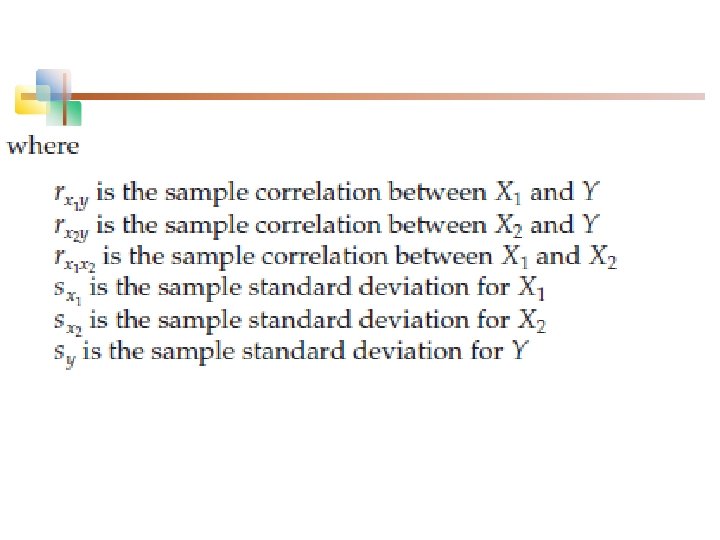
n The coefficient estimators are computed using the following equations:

Example: 2 Independent Variables n A distributor of frozen desert pies wants to evaluate factors thought to influence demand n n n Dependent variable: Pie sales (units per week) Independent variables: Price (in $) Advertising ($100’s) Data are collected for 15 weeks Copyright © 2013 Pearson Education, Inc. Publishing as Prentice Hall Ch. 12 -12

Pie Sales Example Week Pie Sales Price ($) Advertising ($100 s) 1 350 5. 50 3. 3 2 460 7. 50 3. 3 3 350 8. 00 3. 0 4 430 8. 00 4. 5 5 350 6. 80 3. 0 6 380 7. 50 4. 0 7 430 4. 50 3. 0 8 470 6. 40 3. 7 9 450 7. 00 3. 5 10 490 5. 00 4. 0 11 340 7. 20 3. 5 12 300 7. 90 3. 2 13 440 5. 90 4. 0 14 450 5. 00 3. 5 15 300 7. 00 2. 7 Copyright © 2013 Pearson Education, Inc. Publishing as Prentice Hall Multiple regression equation: Sales = b 0 + b 1 (Price) + b 2 (Advertising) Ch. 12 -13

Estimating a Multiple Linear Regression Equation n Excel can be used to generate the coefficients and measures of goodness of fit for multiple regression n Data / Data Analysis / Regression Copyright © 2013 Pearson Education, Inc. Publishing as Prentice Hall Ch. 12 -14

Multiple Regression Output Regression Statistics Multiple R 0. 72213 R Square 0. 52148 Adjusted R Square 0. 44172 Standard Error 47. 46341 Observations ANOVA Regression 15 df SS MS F 2 29460. 027 14730. 013 Residual 12 27033. 306 2252. 776 Total 14 56493. 333 Coefficients Standard Error Intercept 306. 52619 114. 25389 2. 68285 0. 01993 57. 58835 555. 46404 Price -24. 97509 10. 83213 -2. 30565 0. 03979 -48. 57626 -1. 37392 74. 13096 25. 96732 2. 85478 0. 01449 17. 55303 130. 70888 Advertising Copyright © 2013 Pearson Education, Inc. Publishing as Prentice Hall t Stat 6. 53861 Significance F P-value 0. 01201 Lower 95% Upper 95% Ch. 12 -15

The Multiple Regression Equation where Sales is in number of pies per week Price is in $ Advertising is in $100’s. b 1 = -24. 975: sales will decrease, on average, by 24. 975 pies per week for each $1 increase in selling price, net of the effects of changes due to advertising Copyright © 2013 Pearson Education, Inc. Publishing as Prentice Hall b 2 = 74. 131: sales will increase, on average, by 74. 131 pies per week for each $100 increase in advertising, net of the effects of changes due to price Ch. 12 -16

Example 12. 3 n n n n Y profit margines X 1: net revenue for deposit dollar X 2 nunber of offices Y = 1. 56 + 0. 237 X 1 -0. 000249 X 2 Corrleations Y X 1 -0. 704 X 2 -. 0. 868 0. 941

n n Y = 1. 33 -0. 169 X 1 Y = 1. 55 – 0. 000120 X 2

12. 3 Explanatory Power of a Multiple Regression Equation Coefficient of Determination, R 2 n n Reports the proportion of total variation in y explained by all x variables taken together This is the ratio of the explained variability to total sample variability Copyright © 2013 Pearson Education, Inc. Publishing as Prentice Hall Ch. 12 -19

Coefficient of Determination, R 2 Regression Statistics Multiple R 0. 72213 R Square 0. 52148 Adjusted R Square 0. 44172 Standard Error Observations ANOVA Regression 52. 1% of the variation in pie sales is explained by the variation in price and advertising 47. 46341 15 df SS MS F 2 29460. 027 14730. 013 Residual 12 27033. 306 2252. 776 Total 14 56493. 333 Coefficients Standard Error Intercept 306. 52619 114. 25389 2. 68285 0. 01993 57. 58835 555. 46404 Price -24. 97509 10. 83213 -2. 30565 0. 03979 -48. 57626 -1. 37392 74. 13096 25. 96732 2. 85478 0. 01449 17. 55303 130. 70888 Advertising Copyright © 2013 Pearson Education, Inc. Publishing as Prentice Hall t Stat 6. 53861 Significance F P-value 0. 01201 Lower 95% Upper 95% Ch. 12 -20

Estimation of Error Variance n Consider the population regression model n The unbiased estimate of the variance of the errors is where n The square root of the variance, se , is called the standard error of the estimate Copyright © 2013 Pearson Education, Inc. Publishing as Prentice Hall Ch. 12 -21

Standard Error, se Regression Statistics Multiple R 0. 72213 R Square 0. 52148 Adjusted R Square 0. 44172 Standard Error 47. 46341 Observations ANOVA Regression The magnitude of this value can be compared to the average y value 15 df SS MS F 2 29460. 027 14730. 013 Residual 12 27033. 306 2252. 776 Total 14 56493. 333 Coefficients Standard Error Intercept 306. 52619 114. 25389 2. 68285 0. 01993 57. 58835 555. 46404 Price -24. 97509 10. 83213 -2. 30565 0. 03979 -48. 57626 -1. 37392 74. 13096 25. 96732 2. 85478 0. 01449 17. 55303 130. 70888 Advertising Copyright © 2013 Pearson Education, Inc. Publishing as Prentice Hall t Stat 6. 53861 Significance F P-value 0. 01201 Lower 95% Upper 95% Ch. 12 -22

Adjusted Coefficient of Determination, n n R 2 never decreases when a new X variable is added to the model, even if the new variable is not an important predictor variable n This can be a disadvantage when comparing models What is the net effect of adding a new variable? n We lose a degree of freedom when a new X variable is added n Did the new X variable add enough explanatory power to offset the loss of one degree of freedom? Copyright © 2013 Pearson Education, Inc. Publishing as Prentice Hall Ch. 12 -23

Adjusted Coefficient of Determination, (continued) n Used to correct for the fact that adding non-relevant independent variables will still reduce the error sum of squares (where n = sample size, K = number of independent variables) n n n Adjusted R 2 provides a better comparison between multiple regression models with different numbers of independent variables Penalize excessive use of unimportant independent variables Value is less than R 2 Copyright © 2013 Pearson Education, Inc. Publishing as Prentice Hall Ch. 12 -24

Regression Statistics Multiple R 0. 72213 R Square 0. 52148 Adjusted R Square 0. 44172 Standard Error 47. 46341 Observations ANOVA Regression 15 df 44. 2% of the variation in pie sales is explained by the variation in price and advertising, taking into account the sample size and number of independent variables SS MS F 2 29460. 027 14730. 013 Residual 12 27033. 306 2252. 776 Total 14 56493. 333 Coefficients Standard Error Intercept 306. 52619 114. 25389 2. 68285 0. 01993 57. 58835 555. 46404 Price -24. 97509 10. 83213 -2. 30565 0. 03979 -48. 57626 -1. 37392 74. 13096 25. 96732 2. 85478 0. 01449 17. 55303 130. 70888 Advertising Copyright © 2013 Pearson Education, Inc. Publishing as Prentice Hall t Stat 6. 53861 Significance F P-value 0. 01201 Lower 95% Upper 95% Ch. 12 -25

Coefficient of Multiple Correlation n n The coefficient of multiple correlation is the correlation between the predicted value and the observed value of the dependent variable Is the square root of the multiple coefficient of determination Used as another measure of the strength of the linear relationship between the dependent variable and the independent variables Comparable to the correlation between Y and X in simple regression Copyright © 2013 Pearson Education, Inc. Publishing as Prentice Hall Ch. 12 -26

12. 4 Conf. Intervals and Hypothesis Tests for Regression Coefficients The variance of a coefficient estimate is affected by: n n the sample size the spread of the X variables the correlations between the independent variables, and the model error term We are typically more interested in the regression coefficients bj than in the constant or intercept b 0 Copyright © 2013 Pearson Education, Inc. Publishing as Prentice Hall Ch. 12 -27

Confidence Intervals Confidence interval limits for the population slope βj where t has (n – K – 1) d. f. Coefficients Standard Error Intercept 306. 52619 114. 25389 Price -24. 97509 10. 83213 74. 13096 25. 96732 Advertising Here, t has (15 – 2 – 1) = 12 d. f. Example: Form a 95% confidence interval for the effect of changes in price (x 1) on pie sales: -24. 975 ± (2. 1788)(10. 832) So the interval is Copyright © 2013 Pearson Education, Inc. Publishing as Prentice Hall -48. 576 < β 1 < -1. 374 Ch. 12 -28

Confidence Intervals (continued) Confidence interval for the population slope βi Coefficients Standard Error … Intercept 306. 52619 114. 25389 … 57. 58835 555. 46404 Price -24. 97509 10. 83213 … -48. 57626 -1. 37392 74. 13096 25. 96732 … 17. 55303 130. 70888 Advertising Lower 95% Upper 95% Example: Excel output also reports these interval endpoints: Weekly sales are estimated to be reduced by between 1. 37 to 48. 58 pies for each increase of $1 in the selling price Copyright © 2013 Pearson Education, Inc. Publishing as Prentice Hall Ch. 12 -29

Hypothesis Tests n n n Use t-tests for individual coefficients Shows if a specific independent variable is conditionally important Hypotheses: n n H 0: βj = 0 (no linear relationship) H 1: βj ≠ 0 (linear relationship does exist between xj and y) Copyright © 2013 Pearson Education, Inc. Publishing as Prentice Hall Ch. 12 -30

Evaluating Individual Regression Coefficients (continued) H 0: βj = 0 (no linear relationship) H 1: βj ≠ 0 (linear relationship does exist between xi and y) Test Statistic: (df = n – k – 1) Copyright © 2013 Pearson Education, Inc. Publishing as Prentice Hall Ch. 12 -31

Evaluating Individual Regression Coefficients (continued) Regression Statistics Multiple R 0. 72213 R Square 0. 52148 Adjusted R Square 0. 44172 Standard Error 47. 46341 Observations ANOVA Regression 15 df t-value for Price is t = -2. 306, with p-value. 0398 t-value for Advertising is t = 2. 855, with p-value. 0145 SS MS F 2 29460. 027 14730. 013 Residual 12 27033. 306 2252. 776 Total 14 56493. 333 Coefficients Standard Error Intercept 306. 52619 114. 25389 2. 68285 0. 01993 57. 58835 555. 46404 Price -24. 97509 10. 83213 -2. 30565 0. 03979 -48. 57626 -1. 37392 74. 13096 25. 96732 2. 85478 0. 01449 17. 55303 130. 70888 Advertising Copyright © 2013 Pearson Education, Inc. Publishing as Prentice Hall t Stat 6. 53861 Significance F P-value 0. 01201 Lower 95% Upper 95% Ch. 12 -32

Example: Evaluating Individual Regression Coefficients From Excel output: H 0: β j = 0 H 1: β j 0 Coefficients Standard Error -24. 97509 74. 13096 Price Advertising d. f. = 15 -2 -1 = 12 t Stat P-value 10. 83213 -2. 30565 0. 03979 25. 96732 2. 85478 0. 01449 The test statistic for each variable falls in the rejection region (p-values <. 05) =. 05 t 12, . 025 = 2. 1788 Decision: /2=. 025 Reject H 0 for each variable Conclusion: Reject H 0 Do not reject H 0 -tα/2 -2. 1788 0 Reject H 0 tα/2 2. 1788 Copyright © 2013 Pearson Education, Inc. Publishing as Prentice Hall There is evidence that both Price and Advertising affect pie sales at =. 05 Ch. 12 -33

12. 5 Tests on Regression Coefficients Tests on All Coefficients n n F-Test for Overall Significance of the Model Shows if there is a linear relationship between all of the X variables considered together and Y n Use F test statistic n Hypotheses: H 0: β 1 = β 2 = … = βK = 0 (no linear relationship) H 1: at least one βi ≠ 0 (at least one independent variable affects Y) Copyright © 2013 Pearson Education, Inc. Publishing as Prentice Hall Ch. 12 -34

F-Test for Overall Significance n Test statistic: where F has K (numerator) and (n – K – 1) (denominator) degrees of freedom n The decision rule is Copyright © 2013 Pearson Education, Inc. Publishing as Prentice Hall Ch. 12 -35

F-Test for Overall Significance (continued) Regression Statistics Multiple R 0. 72213 R Square 0. 52148 Adjusted R Square 0. 44172 Standard Error 47. 46341 Observations ANOVA Regression 15 df With 2 and 12 degrees of freedom SS MS P-value for the F-Test F 2 29460. 027 14730. 013 Residual 12 27033. 306 2252. 776 Total 14 56493. 333 Coefficients Standard Error Intercept 306. 52619 114. 25389 2. 68285 0. 01993 57. 58835 555. 46404 Price -24. 97509 10. 83213 -2. 30565 0. 03979 -48. 57626 -1. 37392 74. 13096 25. 96732 2. 85478 0. 01449 17. 55303 130. 70888 Advertising Copyright © 2013 Pearson Education, Inc. Publishing as Prentice Hall t Stat 6. 53861 Significance F P-value 0. 01201 Lower 95% Upper 95% Ch. 12 -36

F-Test for Overall Significance (continued) H 0: β 1 = β 2 = 0 H 1: β 1 and β 2 not both zero =. 05 df 1= 2 df 2 = 12 Critical Value: =. 05 Do not reject H 0 Reject H 0 Decision: Since F test statistic is in the rejection region (pvalue <. 05), reject H 0 F = 3. 885 0 Test Statistic: Conclusion: F F. 05 = 3. 885 Copyright © 2013 Pearson Education, Inc. Publishing as Prentice Hall There is evidence that at least one independent variable affects Y Ch. 12 -37

Test on a Subset of Regression Coefficients n Consider a multiple regression model involving variables Xj and Zj , and the null hypothesis that the Z variable coefficients are all zero: Copyright © 2013 Pearson Education, Inc. Publishing as Prentice Hall Ch. 12 -38

Tests on a Subset of Regression Coefficients (continued) n Goal: compare the error sum of squares for the complete model with the error sum of squares for the restricted model n n n First run a regression for the complete model and obtain SSE Next run a restricted regression that excludes the Z variables (the number of variables excluded is R) and obtain the restricted error sum of squares SSE(R) Compute the F statistic and apply the decision rule for a significance level Copyright © 2013 Pearson Education, Inc. Publishing as Prentice Hall Ch. 12 -39

Newbold 12. 41 n n n=30 families Explain household milk consumption Y: milk consumption (quarts per week) X 1: family income (dolars per week) X 2: family size LS estimators : b 0: -0. 025, b 1: 0. 052, b 2: 1. 14 SST: 162. 1, SSE: 88. 2 : X 3: number of preschool childeren ? SSE 83. 7

n n Test the null hypothesis that Number of preschool childeren in a family dose not significantly ieffects weekly family milk consumption

12. 6 n n n Prediction Given a population regression model then given a new observation of a data point (x 1, n+1, x 2, n+1, . . . , x K, n+1) the best linear unbiased forecast of y^n+1 is It is risky to forecast for new X values outside the range of the data used to estimate the model coefficients, because we do not have data to support that the linear model extends beyond the observed range. Copyright © 2013 Pearson Education, Inc. Publishing as Prentice Hall Ch. 12 -43

Predictions from a Multiple Regression Model Predict sales for a week in which the selling price is $5. 50 and advertising is $350: Predicted sales is 428. 62 pies Copyright © 2013 Pearson Education, Inc. Publishing as Prentice Hall Note that Advertising is in $100’s, so $350 means that X 2 = 3. 5 Ch. 12 -44

Transformations for Nonlinear Regression Models 12. 7 n n n The relationship between the dependent variable and an independent variable may not be linear Can review the scatter diagram to check for non-linear relationships Example: Quadratic model n The second independent variable is the square of the first variable Copyright © 2013 Pearson Education, Inc. Publishing as Prentice Hall Ch. 12 -45

Quadratic Model Transformations Quadratic model form: Let And specify the model as n where: β 0 = Y intercept β 1 = regression coefficient for linear effect of X on Y β 2 = regression coefficient for quadratic effect on Y εi = random error in Y for observation i Copyright © 2013 Pearson Education, Inc. Publishing as Prentice Hall Ch. 12 -46

Linear vs. Nonlinear Fit Y Y X X Linear fit does not give random residuals Copyright © 2013 Pearson Education, Inc. Publishing as Prentice Hall residuals X X Nonlinear fit gives random residuals Ch. 12 -47

Quadratic Regression Model Quadratic models may be considered when the scatter diagram takes on one of the following shapes: Y Y β 1 < 0 β 2 > 0 X 1 Y β 1 > 0 β 2 > 0 X 1 Y β 1 < 0 β 2 < 0 X 1 β 1 > 0 β 2 < 0 X 1 β 1 = the coefficient of the linear term β 2 = the coefficient of the squared term Copyright © 2013 Pearson Education, Inc. Publishing as Prentice Hall Ch. 12 -48

Testing for Significance: Quadratic Effect n Testing the Quadratic Effect n Compare the linear regression estimate n with quadratic regression estimate n Hypotheses n H 0: β 2 = 0 (The quadratic term does not improve the model) n H 1: β 2 0 (The quadratic term improves the model) Copyright © 2013 Pearson Education, Inc. Publishing as Prentice Hall Ch. 12 -49

Testing for Significance: Quadratic Effect (continued) n Testing the Quadratic Effect Hypotheses n n H 0 : β 2 = 0 (The quadratic term does not improve the model) n H 1 : β 2 0 (The quadratic term improves the model) The test statistic is where: b 2 = squared term slope coefficient β 2 = hypothesized slope (zero) Sb = standard error of the slope 2 Copyright © 2013 Pearson Education, Inc. Publishing as Prentice Hall Ch. 12 -50

Testing for Significance: Quadratic Effect (continued) n Testing the Quadratic Effect Compare R 2 from simple regression to R 2 from the quadratic model n If R 2 from the quadratic model is larger than R 2 from the simple model, then the quadratic model is a better model Copyright © 2013 Pearson Education, Inc. Publishing as Prentice Hall Ch. 12 -51

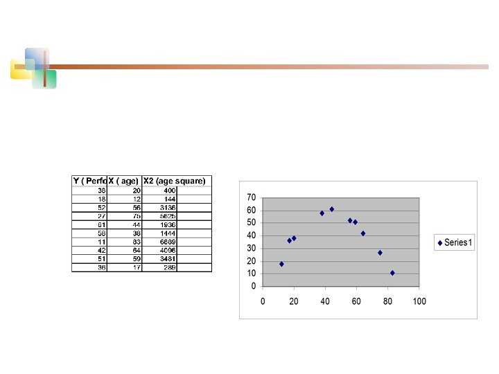
Exmple n n n Performance by age First increases and then falls again for older ages Quadartic relation

Example: Quadratic Model Purity Filter Time 3 1 7 2 8 3 15 5 22 7 33 8 40 10 54 12 67 13 70 14 78 15 85 15 87 16 99 17 n Purity increases as filter time increases: Copyright © 2013 Pearson Education, Inc. Publishing as Prentice Hall Ch. 12 -55

Example: Quadratic Model (continued) n Simple regression results: y^ = -11. 283 + 5. 985 Time Coefficients Standard Error -11. 28267 3. 46805 -3. 25332 0. 00691 5. 98520 0. 30966 19. 32819 2. 078 E-10 Intercept Time t Stat P-value Regression Statistics R Square 0. 96888 Adjusted R Square 0. 96628 Standard Error 6. 15997 F Significance F 373. 57904 2. 0778 E-10 t statistic, F statistic, and R 2 are all high, but the residuals are not random: Copyright © 2013 Pearson Education, Inc. Publishing as Prentice Hall Ch. 12 -56

Example: Quadratic Model (continued) § Quadratic regression results: y^ = 1. 539 + 1. 565 Time + 0. 245 (Time)2 Coefficients Standard Error Intercept 1. 53870 2. 24465 0. 68550 0. 50722 Time 1. 56496 0. 60179 2. 60052 0. 02467 Time-squared 0. 24516 0. 03258 7. 52406 1. 165 E-05 Regression Statistics R Square 0. 99494 Adjusted R Square 0. 99402 Standard Error 2. 59513 t Stat F P-value Significance F 1080. 7330 2. 368 E-13 The quadratic term is significant and improves the model: R 2 is higher and se is lower, residuals are now random Copyright © 2013 Pearson Education, Inc. Publishing as Prentice Hall Ch. 12 -57

Interpretation of coefficients For the logarithmic model: n When both dependent and independent variables are logged: n The estimated coefficient bk of the independent variable Xk can be interpreted as a 1 percent change in Xk leads to an estimated bk percentage change in the average value of Y n bk is the elasticity of Y with respect to a change in Xk Copyright © 2013 Pearson Education, Inc. Publishing as Prentice Hall Ch. 12 -59

Example Cobb-Douglas Production Function n Production function output as a function of labor and capital

Original and new Variables n Original data and new variables

Regression Output

Parameter valeus n n n b 1 =0. 71 B 2= 1 - 0. 71 = 0. 29 Ln(b 0) = 2. 577 so b 0 = exp(2. 577) = 13. 15 The estimated cobb-douglas Prodcution Function is Output = 13. 15*L 0. 71 K 0. 29,

Dummy Variables for Regression Models 12. 8 n A dummy variable is a categorical independent variable with two levels: n n n yes or no, on or off, male or female recorded as 0 or 1 Regression intercepts are different if the variable is significant Assumes equal slopes for other variables If more than two levels, the number of dummy variables needed is (number of levels - 1) Copyright © 2013 Pearson Education, Inc. Publishing as Prentice Hall Ch. 12 -64

Dummy Variable Example Let: y = Pie Sales x 1 = Price x 2 = Holiday (X 2 = 1 if a holiday occurred during the week) (X 2 = 0 if there was no holiday that week) Copyright © 2013 Pearson Education, Inc. Publishing as Prentice Hall Ch. 12 -65

Dummy Variable Example (continued) Holiday No Holiday Different intercept y (sales) b 0 + b 2 b 0 Holi da y (x 2 No H o liday = 1) (x 2 = 0) Copyright © 2013 Pearson Education, Inc. Publishing as Prentice Hall Same slope If H 0: β 2 = 0 is rejected, then “Holiday” has a significant effect on pie sales x 1 (Price) Ch. 12 -66

Interpreting the Dummy Variable Coefficient Example: Sales: number of pies sold per week Price: pie price in $ 1 If a holiday occurred during the week Holiday: 0 If no holiday occurred b 2 = 15: on average, sales were 15 pies greater in weeks with a holiday than in weeks without a holiday, given the same price Copyright © 2013 Pearson Education, Inc. Publishing as Prentice Hall Ch. 12 -67

Differences in Slope n Hypothesizes interaction between pairs of x variables n n Response to one x variable may vary at different levels of another x variable Contains two-way cross product terms n Copyright © 2013 Pearson Education, Inc. Publishing as Prentice Hall Ch. 12 -68

Effect of Interaction n n Given: Without interaction term, effect of X 1 on Y is measured by β 1 With interaction term, effect of X 1 on Y is measured by β 1 + β 3 X 2 Effect changes as X 2 changes Copyright © 2013 Pearson Education, Inc. Publishing as Prentice Hall Ch. 12 -69

Interaction Example Suppose x 2 is a dummy variable and the estimated regression equation is y 12 x 2 = 1: ^y = 1 + 2 x + 3(1) + 4 x (1) = 4 + 6 x 1 1 1 8 4 x 2 = 0: ^y = 1 + 2 x + 3(0) + 4 x (0) = 1 + 2 x 1 1 1 0 0 0. 5 1 1. 5 x 1 Slopes are different if the effect of x 1 on y depends on x 2 value Copyright © 2013 Pearson Education, Inc. Publishing as Prentice Hall Ch. 12 -70

Significance of Interaction Term n n n The coefficient b 3 is an estimate of the difference in the coefficient of x 1 when x 2 = 1 compared to when x 2 = 0 The t statistic for b 3 can be used to test the hypothesis If we reject the null hypothesis we conclude that there is a difference in the slope coefficient for the two subgroups Copyright © 2013 Pearson Education, Inc. Publishing as Prentice Hall Ch. 12 -71

12. 9 Multiple Regression Analysis Application Procedure Errors (residuals) from the regression model: < ei = (yi – yi) Assumptions: n The errors are normally distributed n Errors have a constant variance n The model errors are independent Copyright © 2013 Pearson Education, Inc. Publishing as Prentice Hall Ch. 12 -72

Analysis of Residuals n These residual plots are used in multiple regression: < n Residuals vs. yi n Residuals vs. x 1 i n Residuals vs. x 2 i n Residuals vs. time (if time series data) Use the residual plots to check for violations of regression assumptions Copyright © 2013 Pearson Education, Inc. Publishing as Prentice Hall Ch. 12 -73

Chapter Summary n n n n n Developed the multiple regression model Tested the significance of the multiple regression model Discussed adjusted R 2 ( R 2 ) Tested individual regression coefficients Tested portions of the regression model Used quadratic terms and log transformations in regression models Explained dummy variables Evaluated interaction effects Discussed using residual plots to check model assumptions Copyright © 2013 Pearson Education, Inc. Publishing as Prentice Hall Ch. 12 -74

Rcrtv, dr 12. 78 n n n=93 rate scale of 1(low)-10(high) n n levels of satisfactions n n n opinion of residence hall life room mates, floor, hall, resident advisor Y. overall opinion X 1, X 4

n n n n n Source model error total param inter. x 1 x 2 x 3 x 4 df SS MSS F 4 37. 016 9. 2540 9. 958 88 81. 780 0. 9293 92 118. 79 estimate t std error 3. 950 5. 84 0. 676 0. 106 1. 69 0. 063 0. 122 1. 70 0. 072 0. 092 1. 75 0. 053 0. 169 2. 64 0. 064 R-sq 0. 312

Exercise 12. 82 n n n developing countiry - 48 countries Y: per manifacturing growth x 1 per agricultural growth x 2 per exorts growth x 3 per rate of inflation

All rights reserved. No part of this publication may be reproduced, stored in a retrieval system, or transmitted, in any form or by any means, electronic, mechanical, photocopying, recording, or otherwise, without the prior written permission of the publisher. Printed in the United States of America. Copyright © 2013 Pearson Education, Inc. Publishing as Prentice Hall Ch. 12 -81

13. 2 n n Dummy Variables and Experimental Design Dummy variables can be used in situations in which the categorical variable of interest has more than two categories Dummy variables can also be useful in experimental design n Experimental design is used to identify possible causes of variation in the value of the dependent variable n Y outcomes are measured at specific combinations of levels for treatment and blocking variables n The goal is to determine how the different treatments influence the Y outcome Copyright © 2013 Pearson Education, Inc. Publishing as Prentice Hall Ch. 13 -83

Dummy Variable Models (More than 2 Levels) n n Consider a categorical variable with K levels The number of dummy variables needed is one less than the number of levels, K – 1 Example: y = house price ; x 1 = square feet If style of the house is also thought to matter: Style = ranch, split level, condo Three levels, so two dummy variables are needed Copyright © 2013 Pearson Education, Inc. Publishing as Prentice Hall Ch. 13 -84

Dummy Variable Models (More than 2 Levels) (continued) n Example: Let “condo” be the default category, and let x 2 and x 3 be used for the other two categories: y = house price x 1 = square feet x 2 = 1 if ranch, 0 otherwise x 3 = 1 if split level, 0 otherwise The multiple regression equation is: Copyright © 2013 Pearson Education, Inc. Publishing as Prentice Hall Ch. 13 -85

Interpreting the Dummy Variable Coefficients (with 3 Levels) Consider the regression equation: For a condo: x 2 = x 3 = 0 For a ranch: x 2 = 1; x 3 = 0 For a split level: x 2 = 0; x 3 = 1 Copyright © 2013 Pearson Education, Inc. Publishing as Prentice Hall With the same square feet, a ranch will have an estimated average price of 23. 53 thousand dollars more than a condo With the same square feet, a split-level will have an estimated average price of 18. 84 thousand dollars more than a condo. Ch. 13 -86

Experimental Design n Consider an experiment in which n n n four treatments will be used, and the outcome also depends on three environmental factors that cannot be controlled by the experimenter Let variable z 1 denote the treatment, where z 1 = 1, 2, 3, or 4. Let z 2 denote the environment factor (the “blocking variable”), where z 2 = 1, 2, or 3 To model the four treatments, three dummy variables are needed To model the three environmental factors, two dummy variables are needed Copyright © 2013 Pearson Education, Inc. Publishing as Prentice Hall Ch. 13 -87

Experimental Design (continued) n Define five dummy variables, x 1, x 2, x 3, x 4, and x 5 n Let treatment level 1 be the default (z 1 = 1) n n Define x 1 = 1 if z 1 = 2, x 1 = 0 otherwise Define x 2 = 1 if z 1 = 3, x 2 = 0 otherwise Define x 3 = 1 if z 1 = 4, x 3 = 0 otherwise Let environment level 1 be the default (z 2 = 1) n n Define x 4 = 1 if z 2 = 2, x 4 = 0 otherwise Define x 5 = 1 if z 2 = 3, x 5 = 0 otherwise Copyright © 2013 Pearson Education, Inc. Publishing as Prentice Hall Ch. 13 -88

Experimental Design: Dummy Variable Tables n The dummy variable values can be summarized in a table: Z 1 X 2 X 3 Z 2 X 4 X 5 1 0 0 0 1 0 0 2 1 0 3 0 1 4 0 0 1 Copyright © 2013 Pearson Education, Inc. Publishing as Prentice Hall Ch. 13 -89

Experimental Design Model n n The experimental design model can be estimated using the equation The estimated value for β 2 , for example, shows the amount by which the y value for treatment 3 exceeds the value for treatment 1 Copyright © 2013 Pearson Education, Inc. Publishing as Prentice Hall Ch. 13 -90

Exercise 13. 3 Write the model specification and define the variables for a multiple regression model to predict the cost per unit produced as a function of factory type indicated as: • classic technology, computer-controlled machines, and computer-controlled material handling), n and as a function of country indicated as n n Colombia, South Africa, and Japan

Solution