MIS 331 Data Mining 20182019 Fall Chapter 8

MIS 331 Data Mining 2018/2019 Fall Chapter 8 Sampliing Distribution, Confidence Interval Estimation and Hypothesis Testing for Variance of a Population Copyright © 2013 Pearson Education, Inc. Publishing as Prentice Hall Ch. 6 -1

Outline n Tests of Equality of Two Variances

Statistics for Business and Economics 8 th Edition Chapter 10 Hypothesis Testing: Additional Topics Copyright © 2013 Pearson Education, Inc. Publishing as Prentice Hall Ch. 10 -3

Chapter Goals After completing this chapter, you should be able to: n Test hypotheses for the difference between two population means n Two means, matched pairs n Independent populations, population variances known n n Independent populations, population variances unknown but equal Complete a hypothesis test for the difference between two proportions (large samples) n Use the F table to find critical F values n Complete an F test for the equality of two variances Copyright © 2013 Pearson Education, Inc. Publishing as Prentice Hall Ch. 10 -4

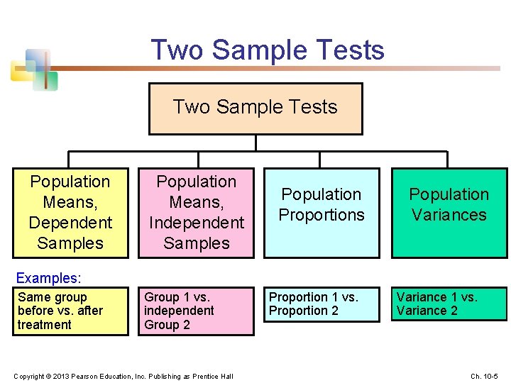
Two Sample Tests Population Means, Dependent Samples Population Means, Independent Samples Population Proportions Population Variances Examples: Same group before vs. after treatment Group 1 vs. independent Group 2 Copyright © 2013 Pearson Education, Inc. Publishing as Prentice Hall Proportion 1 vs. Proportion 2 Variance 1 vs. Variance 2 Ch. 10 -5

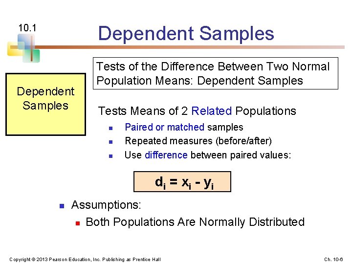
Dependent Samples 10. 1 Dependent Samples Tests of the Difference Between Two Normal Population Means: Dependent Samples Tests Means of 2 Related Populations n n n Paired or matched samples Repeated measures (before/after) Use difference between paired values: d i = x i - yi n Assumptions: n Both Populations Are Normally Distributed Copyright © 2013 Pearson Education, Inc. Publishing as Prentice Hall Ch. 10 -6

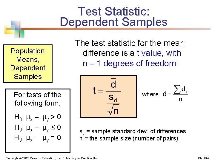
Test Statistic: Dependent Samples Population Means, Dependent Samples The test statistic for the mean difference is a t value, with n – 1 degrees of freedom: For tests of the following form: H 0: μ x – μ y 0 H 0: μ x – μ y ≤ 0 H 0: μ x – μ y = 0 where sd = sample standard dev. of differences n = the sample size (number of pairs) Copyright © 2013 Pearson Education, Inc. Publishing as Prentice Hall Ch. 10 -7

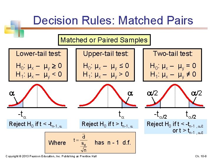
Decision Rules: Matched Pairs Matched or Paired Samples Lower-tail test: Upper-tail test: Two-tail test: H 0: μ x – μ y 0 H 1: μ x – μ y < 0 H 0: μ x – μ y ≤ 0 H 1: μ x – μ y > 0 H 0: μ x – μ y = 0 H 1: μ x – μ y ≠ 0 -t t Reject H 0 if t < -tn-1, Where Reject H 0 if t > tn-1, /2 -t /2 Reject H 0 if t < -tn-1 , /2 or t > tn-1 , /2 has n - 1 d. f. Copyright © 2013 Pearson Education, Inc. Publishing as Prentice Hall Ch. 10 -8

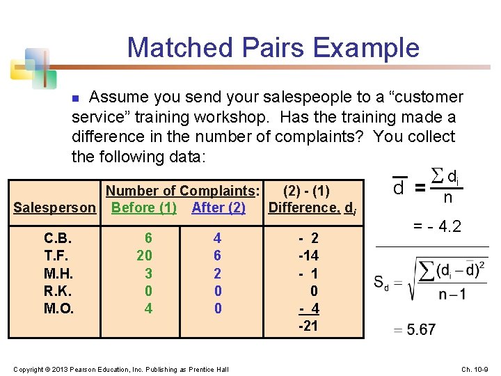
Matched Pairs Example Assume you send your salespeople to a “customer service” training workshop. Has the training made a difference in the number of complaints? You collect the following data: di d = n Number of Complaints: (2) - (1) n Salesperson C. B. T. F. M. H. R. K. M. O. Before (1) 6 20 3 0 4 After (2) 4 6 2 0 0 Copyright © 2013 Pearson Education, Inc. Publishing as Prentice Hall Difference, di - 2 -14 - 1 0 - 4 -21 = - 4. 2 Ch. 10 -9

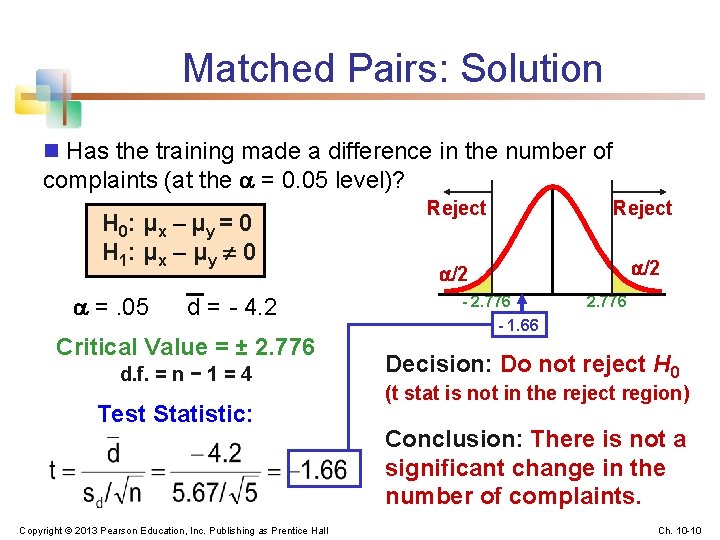
Matched Pairs: Solution n Has the training made a difference in the number of complaints (at the = 0. 05 level)? H 0: μ x – μ y = 0 H 1: μ x – μ y 0 =. 05 d = - 4. 2 Critical Value = ± 2. 776 d. f. = n − 1 = 4 Test Statistic: Copyright © 2013 Pearson Education, Inc. Publishing as Prentice Hall Reject /2 - 2. 776 - 1. 66 2. 776 Decision: Do not reject H 0 (t stat is not in the reject region) Conclusion: There is not a significant change in the number of complaints. Ch. 10 -10

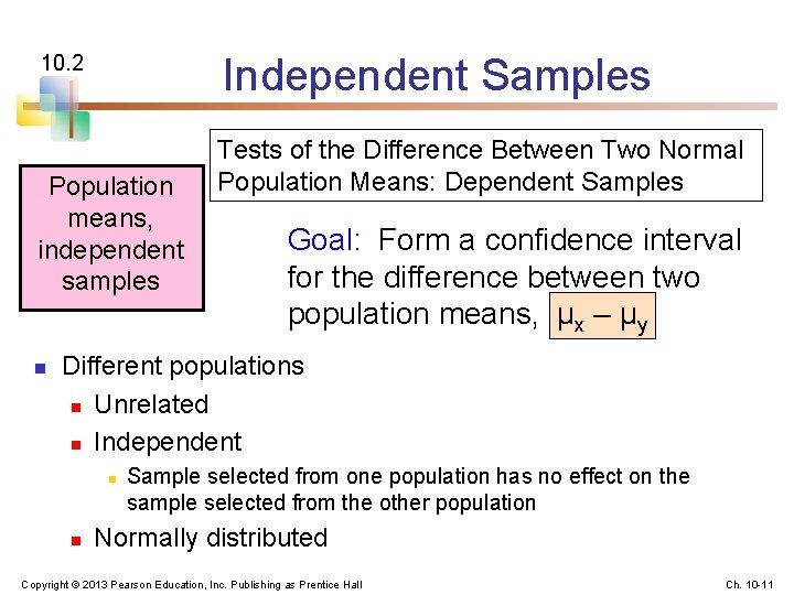
Independent Samples 10. 2 Population means, independent samples n Tests of the Difference Between Two Normal Population Means: Dependent Samples Goal: Form a confidence interval for the difference between two population means, μx – μy Different populations n Unrelated n Independent n n Sample selected from one population has no effect on the sample selected from the other population Normally distributed Copyright © 2013 Pearson Education, Inc. Publishing as Prentice Hall Ch. 10 -11

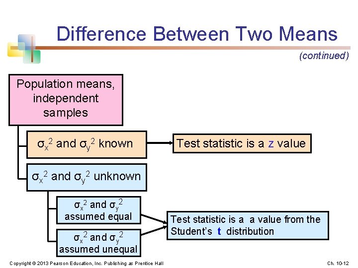
Difference Between Two Means (continued) Population means, independent samples σx 2 and σy 2 known Test statistic is a z value σx 2 and σy 2 unknown σx 2 and σy 2 assumed equal σx 2 and σy 2 assumed unequal Copyright © 2013 Pearson Education, Inc. Publishing as Prentice Hall Test statistic is a a value from the Student’s t distribution Ch. 10 -12

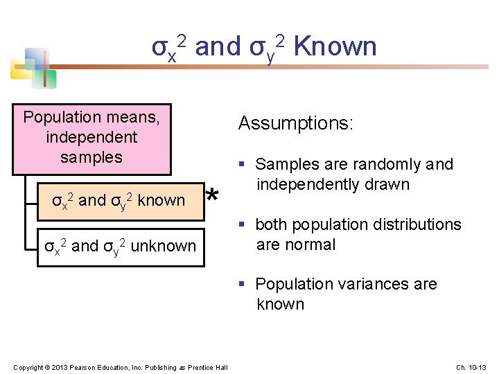
σx 2 and σy 2 Known Population means, independent samples σx 2 and σy 2 known Assumptions: * σx 2 and σy 2 unknown § Samples are randomly and independently drawn § both population distributions are normal § Population variances are known Copyright © 2013 Pearson Education, Inc. Publishing as Prentice Hall Ch. 10 -13

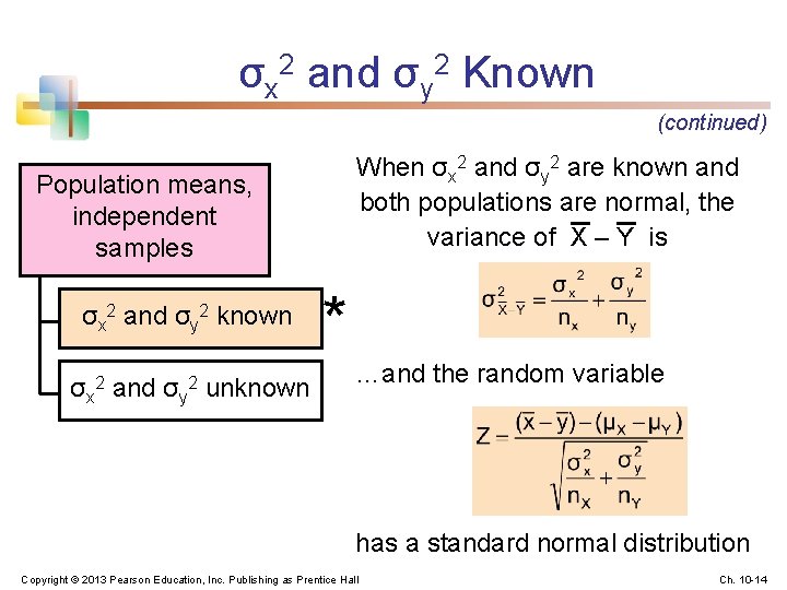
σx 2 and σy 2 Known (continued) When σx 2 and σy 2 are known and both populations are normal, the variance of X – Y is Population means, independent samples σx 2 and σy 2 known σx 2 and σy 2 unknown * …and the random variable has a standard normal distribution Copyright © 2013 Pearson Education, Inc. Publishing as Prentice Hall Ch. 10 -14

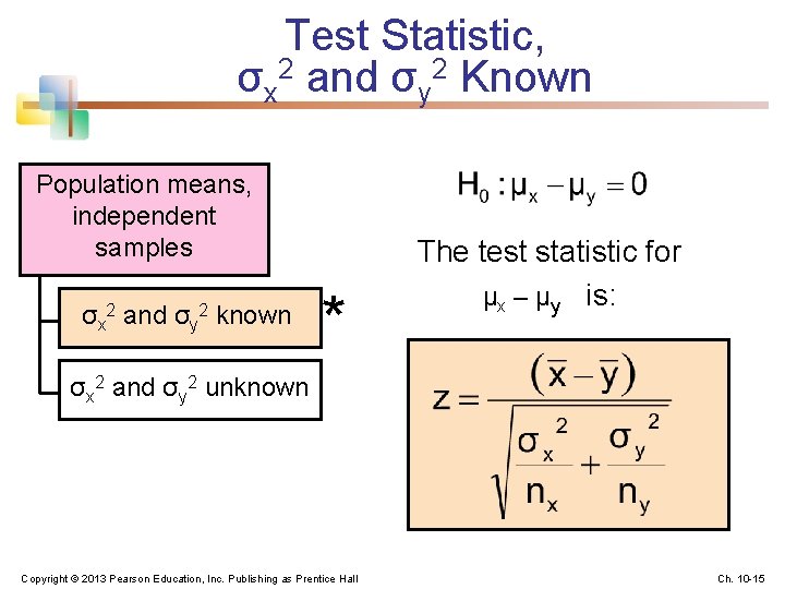
Test Statistic, σx 2 and σy 2 Known Population means, independent samples σx 2 and σy 2 known * The test statistic for μx – μy is: σx 2 and σy 2 unknown Copyright © 2013 Pearson Education, Inc. Publishing as Prentice Hall Ch. 10 -15

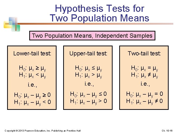
Hypothesis Tests for Two Population Means, Independent Samples Lower-tail test: Upper-tail test: Two-tail test: H 0: μ x μ y H 1: μ x < μ y H 0: μ x ≤ μ y H 1: μ x > μ y H 0: μ x = μ y H 1: μ x ≠ μ y i. e. , H 0: μ x – μ y 0 H 1: μ x – μ y < 0 H 0: μ x – μ y ≤ 0 H 1: μ x – μ y > 0 H 0: μ x – μ y = 0 H 1: μ x – μ y ≠ 0 Copyright © 2013 Pearson Education, Inc. Publishing as Prentice Hall Ch. 10 -16

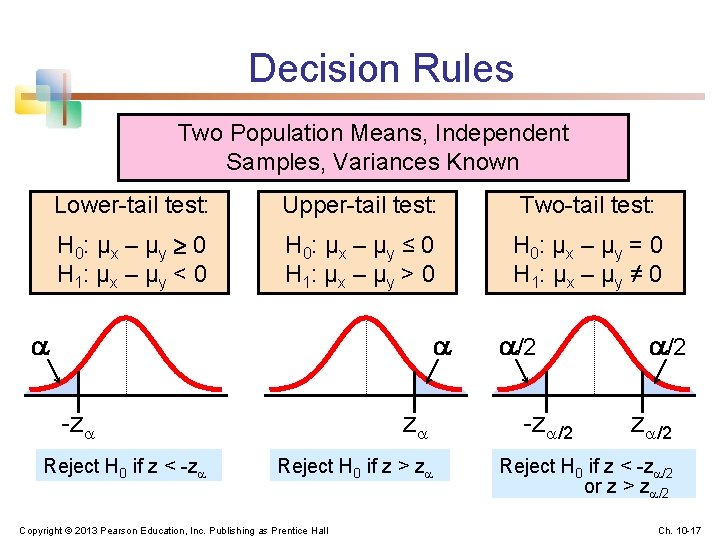
Decision Rules Two Population Means, Independent Samples, Variances Known Lower-tail test: Upper-tail test: Two-tail test: H 0: μ x – μ y 0 H 1: μ x – μ y < 0 H 0: μ x – μ y ≤ 0 H 1: μ x – μ y > 0 H 0: μ x – μ y = 0 H 1: μ x – μ y ≠ 0 -z Reject H 0 if z < -z z Reject H 0 if z > z Copyright © 2013 Pearson Education, Inc. Publishing as Prentice Hall /2 -z /2 Reject H 0 if z < -z /2 or z > z /2 Ch. 10 -17

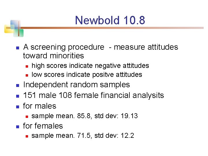
Newbold 10. 8 n A screening procedure - measure attitudes toward minorities n n n Independent random samples 151 male 108 female financial analysits for males n n high scores indicate negative attitudes low scores indicate positve attitudes sample mean. 85. 8, std dev: 19. 13 for females n sample mean. 71. 5, std dev: 12. 2

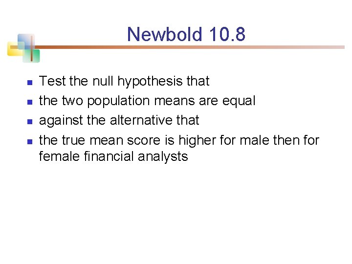
Newbold 10. 8 n n Test the null hypothesis that the two population means are equal against the alternative that the true mean score is higher for male then for female financial analysts

Solution

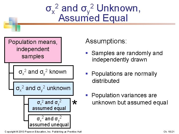
σx 2 and σy 2 Unknown, Assumed Equal Assumptions: Population means, independent samples § Samples are randomly and independently drawn σx 2 and σy 2 known § Populations are normally distributed σx 2 and σy 2 unknown σx 2 and σy 2 assumed equal * § Population variances are unknown but assumed equal σx 2 and σy 2 assumed unequal Copyright © 2013 Pearson Education, Inc. Publishing as Prentice Hall Ch. 10 -21

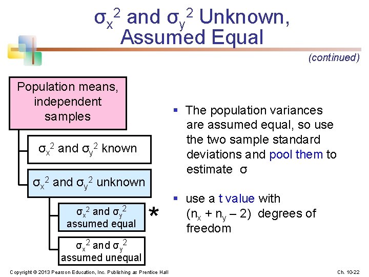
σx 2 and σy 2 Unknown, Assumed Equal (continued) Population means, independent samples § The population variances are assumed equal, so use the two sample standard deviations and pool them to estimate σ σx 2 and σy 2 known σx 2 and σy 2 unknown σx 2 and σy 2 assumed equal * § use a t value with (nx + ny – 2) degrees of freedom σx 2 and σy 2 assumed unequal Copyright © 2013 Pearson Education, Inc. Publishing as Prentice Hall Ch. 10 -22

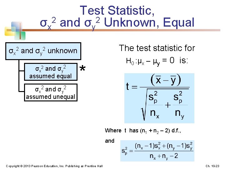
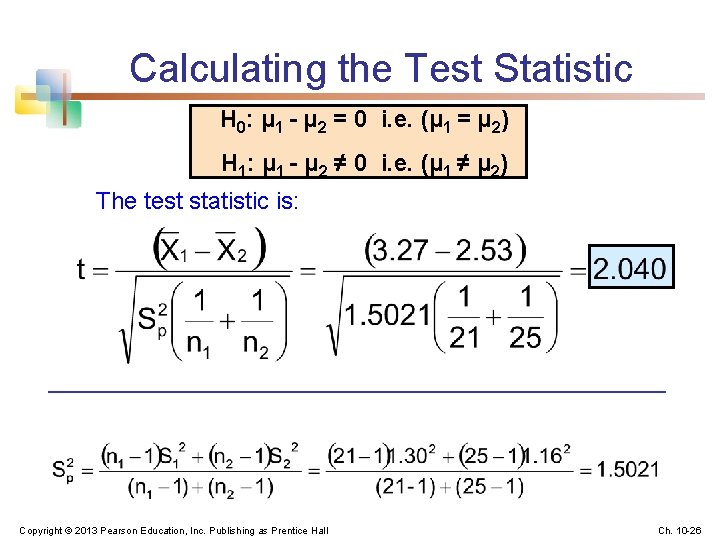
Test Statistic, σx 2 and σy 2 Unknown, Equal The test statistic for H 0 : μx – μy = 0 is: σx 2 and σy 2 unknown σx 2 and σy 2 assumed equal * σx 2 and σy 2 assumed unequal Where t has (n 1 + n 2 – 2) d. f. , and Copyright © 2013 Pearson Education, Inc. Publishing as Prentice Hall Ch. 10 -23

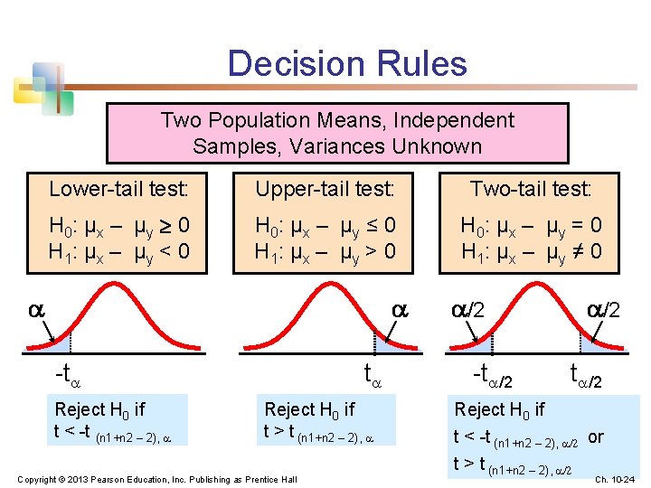
Decision Rules Two Population Means, Independent Samples, Variances Unknown Lower-tail test: Upper-tail test: Two-tail test: H 0: μ x – μ y 0 H 1: μ x – μ y < 0 H 0: μ x – μ y ≤ 0 H 1: μ x – μ y > 0 H 0: μ x – μ y = 0 H 1: μ x – μ y ≠ 0 -t Reject H 0 if t < -t (n 1+n 2 – 2), t Reject H 0 if t > t (n 1+n 2 – 2), Copyright © 2013 Pearson Education, Inc. Publishing as Prentice Hall /2 -t /2 Reject H 0 if t < -t (n 1+n 2 – 2), /2 or t > t (n 1+n 2 – 2), /2 Ch. 10 -24

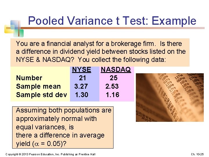
Pooled Variance t Test: Example You are a financial analyst for a brokerage firm. Is there a difference in dividend yield between stocks listed on the NYSE & NASDAQ? You collect the following data: NYSE NASDAQ Number 21 25 Sample mean 3. 27 2. 53 Sample std dev 1. 30 1. 16 Assuming both populations are approximately normal with equal variances, is there a difference in average yield ( = 0. 05)? Copyright © 2013 Pearson Education, Inc. Publishing as Prentice Hall Ch. 10 -25

Calculating the Test Statistic H 0: μ 1 - μ 2 = 0 i. e. (μ 1 = μ 2) H 1: μ 1 - μ 2 ≠ 0 i. e. (μ 1 ≠ μ 2) The test statistic is: Copyright © 2013 Pearson Education, Inc. Publishing as Prentice Hall Ch. 10 -26

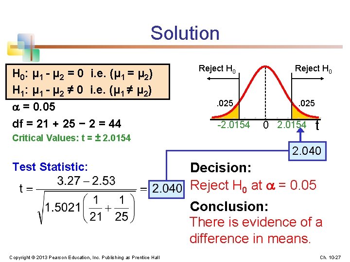
Solution H 0: μ 1 - μ 2 = 0 i. e. (μ 1 = μ 2) H 1: μ 1 - μ 2 ≠ 0 i. e. (μ 1 ≠ μ 2) = 0. 05 df = 21 + 25 − 2 = 44 Critical Values: t = ± 2. 0154 Reject H 0 . 025 -2. 0154 Reject H 0 . 025 0 2. 0154 t 2. 040 Test Statistic: Decision: Reject H 0 at = 0. 05 Conclusion: There is evidence of a difference in means. Copyright © 2013 Pearson Education, Inc. Publishing as Prentice Hall Ch. 10 -27

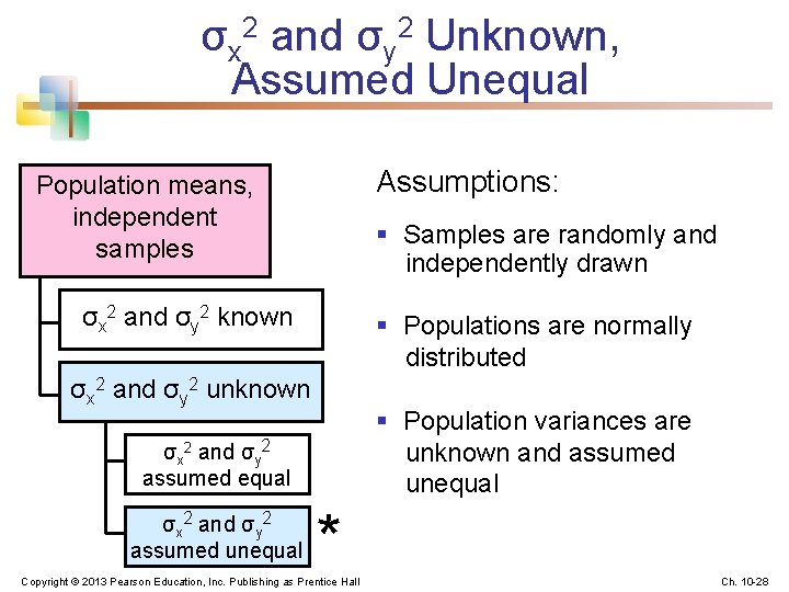
σx 2 and σy 2 Unknown, Assumed Unequal Assumptions: Population means, independent samples § Samples are randomly and independently drawn σx 2 and σy 2 known § Populations are normally distributed σx 2 and σy 2 unknown § Population variances are unknown and assumed unequal σx 2 and σy 2 assumed unequal * Copyright © 2013 Pearson Education, Inc. Publishing as Prentice Hall Ch. 10 -28

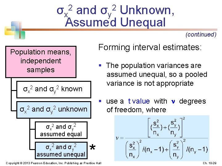
σx 2 and σy 2 Unknown, Assumed Unequal (continued) Forming interval estimates: Population means, independent samples § The population variances are assumed unequal, so a pooled variance is not appropriate σx 2 and σy 2 known § use a t value with degrees of freedom, where σx 2 and σy 2 unknown σx 2 and σy 2 assumed equal σx 2 and σy 2 assumed unequal * Copyright © 2013 Pearson Education, Inc. Publishing as Prentice Hall Ch. 10 -29

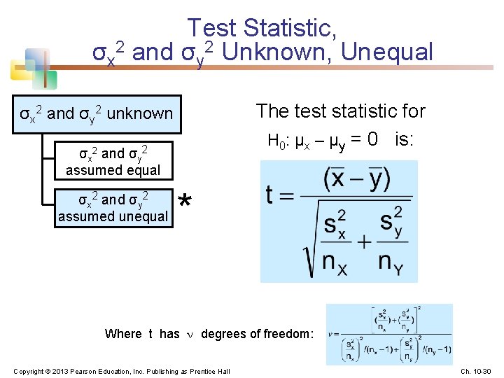
Test Statistic, σx 2 and σy 2 Unknown, Unequal The test statistic for H 0: μx – μy = 0 is: σx 2 and σy 2 unknown σx 2 and σy 2 assumed equal σx 2 and σy 2 assumed unequal * Where t has degrees of freedom: Copyright © 2013 Pearson Education, Inc. Publishing as Prentice Hall Ch. 10 -30

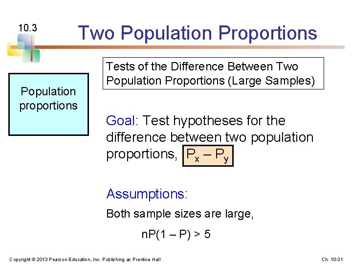
10. 3 Population proportions Two Population Proportions Tests of the Difference Between Two Population Proportions (Large Samples) Goal: Test hypotheses for the difference between two population proportions, Px – Py Assumptions: Both sample sizes are large, n. P(1 – P) > 5 Copyright © 2013 Pearson Education, Inc. Publishing as Prentice Hall Ch. 10 -31

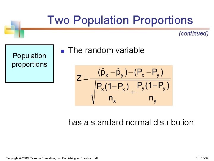
Two Population Proportions (continued) Population proportions n The random variable has a standard normal distribution Copyright © 2013 Pearson Education, Inc. Publishing as Prentice Hall Ch. 10 -32

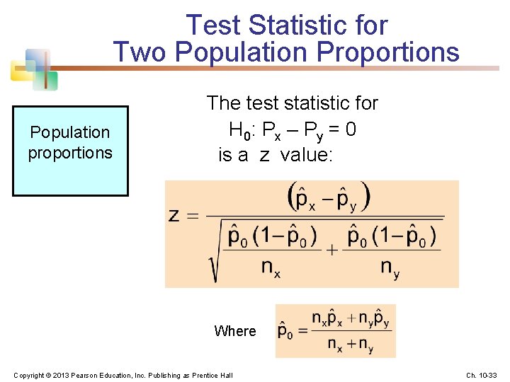
Test Statistic for Two Population Proportions Population proportions The test statistic for H 0: P x – P y = 0 is a z value: Where Copyright © 2013 Pearson Education, Inc. Publishing as Prentice Hall Ch. 10 -33

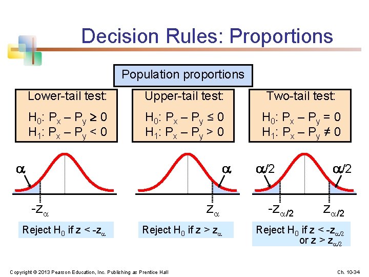
Decision Rules: Proportions Population proportions Lower-tail test: Upper-tail test: Two-tail test: H 0: P x – P y 0 H 1: P x – P y < 0 H 0: P x – P y ≤ 0 H 1: P x – P y > 0 H 0: P x – P y = 0 H 1: P x – P y ≠ 0 -z Reject H 0 if z < -z z Reject H 0 if z > z Copyright © 2013 Pearson Education, Inc. Publishing as Prentice Hall /2 -z /2 Reject H 0 if z < -z /2 or z > z /2 Ch. 10 -34

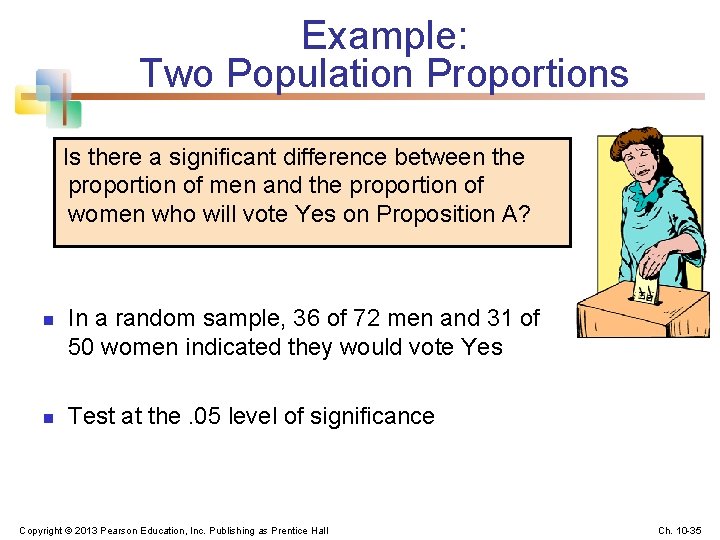
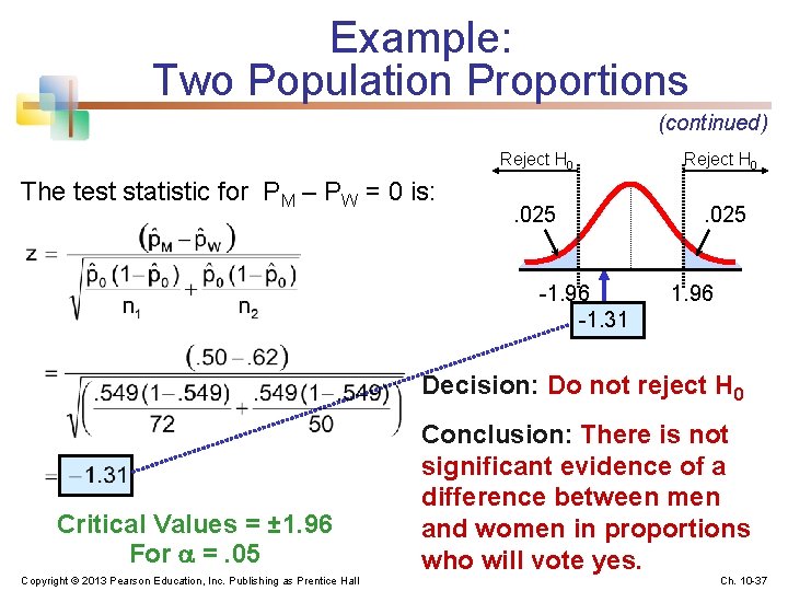
Example: Two Population Proportions Is there a significant difference between the proportion of men and the proportion of women who will vote Yes on Proposition A? n n In a random sample, 36 of 72 men and 31 of 50 women indicated they would vote Yes Test at the. 05 level of significance Copyright © 2013 Pearson Education, Inc. Publishing as Prentice Hall Ch. 10 -35

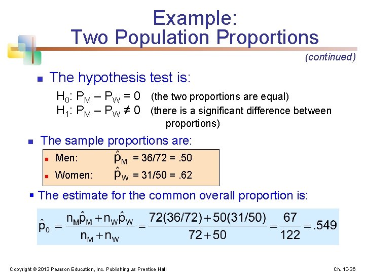
Example: Two Population Proportions (continued) The hypothesis test is: n H 0: PM – PW = 0 (the two proportions are equal) H 1: PM – PW ≠ 0 (there is a significant difference between proportions) n The sample proportions are: n Men: = 36/72 =. 50 n Women: = 31/50 =. 62 § The estimate for the common overall proportion is: Copyright © 2013 Pearson Education, Inc. Publishing as Prentice Hall Ch. 10 -36

Example: Two Population Proportions (continued) The test statistic for PM – PW = 0 is: Reject H 0 . 025 -1. 96 -1. 31 1. 96 Decision: Do not reject H 0 Critical Values = ± 1. 96 For =. 05 Copyright © 2013 Pearson Education, Inc. Publishing as Prentice Hall Conclusion: There is not significant evidence of a difference between men and women in proportions who will vote yes. Ch. 10 -37

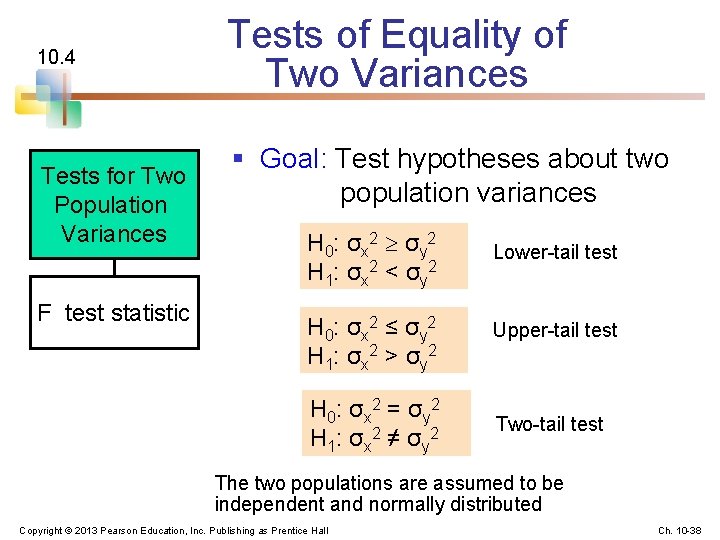
10. 4 Tests for Two Population Variances F test statistic Tests of Equality of Two Variances § Goal: Test hypotheses about two population variances H 0: σx 2 σy 2 H 1: σx 2 < σy 2 H 0: σx 2 ≤ σy 2 H 1: σx 2 > σy 2 H 0: σx 2 = σy 2 H 1: σx 2 ≠ σy 2 Lower-tail test Upper-tail test Two-tail test The two populations are assumed to be independent and normally distributed Copyright © 2013 Pearson Education, Inc. Publishing as Prentice Hall Ch. 10 -38

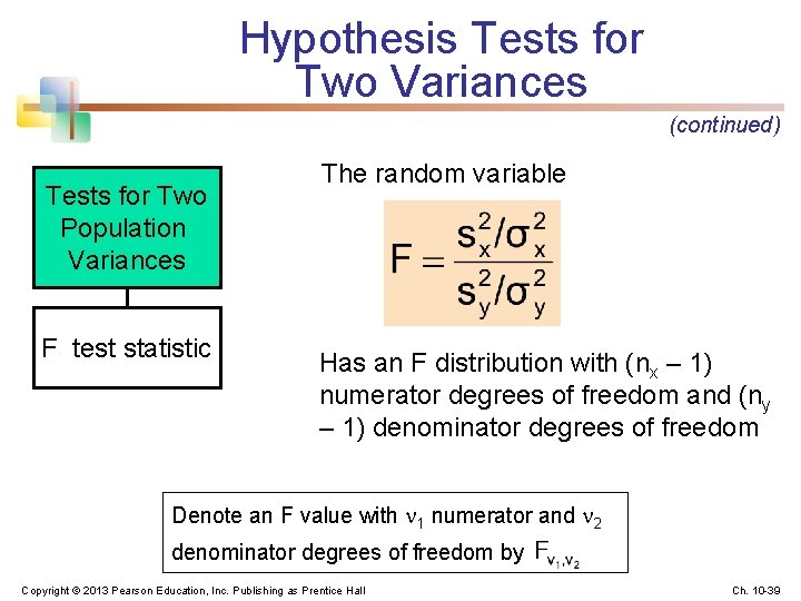
Hypothesis Tests for Two Variances (continued) Tests for Two Population Variances F test statistic The random variable Has an F distribution with (nx – 1) numerator degrees of freedom and (ny – 1) denominator degrees of freedom Denote an F value with 1 numerator and 2 denominator degrees of freedom by Copyright © 2013 Pearson Education, Inc. Publishing as Prentice Hall Ch. 10 -39

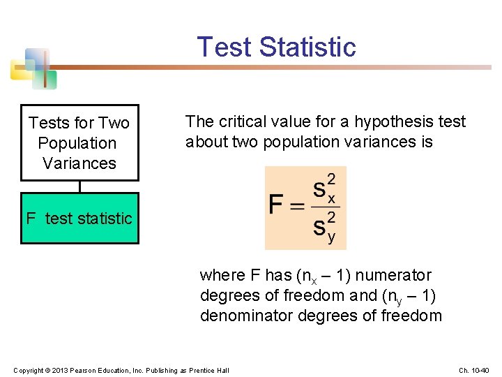
Test Statistic Tests for Two Population Variances The critical value for a hypothesis test about two population variances is F test statistic where F has (nx – 1) numerator degrees of freedom and (ny – 1) denominator degrees of freedom Copyright © 2013 Pearson Education, Inc. Publishing as Prentice Hall Ch. 10 -40

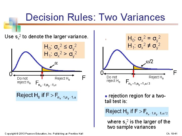
Decision Rules: Two Variances Use sx 2 to denote the larger variance. H 0: σx 2 = σy 2 H 1: σx 2 ≠ σy 2 H 0: σx 2 ≤ σy 2 H 1: σx 2 > σy 2 /2 0 Do not reject H 0 Reject H 0 F 0 Do not reject H 0 F Reject H 0 rejection region for a twotail test is: n where sx 2 is the larger of the two sample variances Copyright © 2013 Pearson Education, Inc. Publishing as Prentice Hall Ch. 10 -41

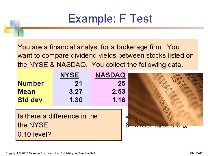
Example: F Test You are a financial analyst for a brokerage firm. You want to compare dividend yields between stocks listed on the NYSE & NASDAQ. You collect the following data: NYSE NASDAQ Number 21 25 Mean 3. 27 2. 53 Std dev 1. 30 1. 16 Is there a difference in the NYSE 0. 10 level? Copyright © 2013 Pearson Education, Inc. Publishing as Prentice Hall variances between & NASDAQ at the = Ch. 10 -42

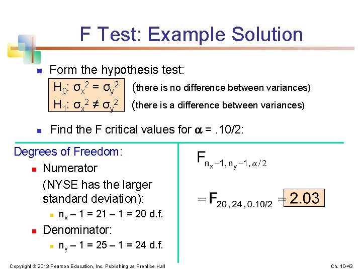
F Test: Example Solution n n Form the hypothesis test: H 0: σx 2 = σy 2 (there is no difference between variances) H 1: σx 2 ≠ σy 2 (there is a difference between variances) Find the F critical values for =. 10/2: Degrees of Freedom: n Numerator (NYSE has the larger standard deviation): n n nx – 1 = 21 – 1 = 20 d. f. Denominator: n ny – 1 = 25 – 1 = 24 d. f. Copyright © 2013 Pearson Education, Inc. Publishing as Prentice Hall Ch. 10 -43

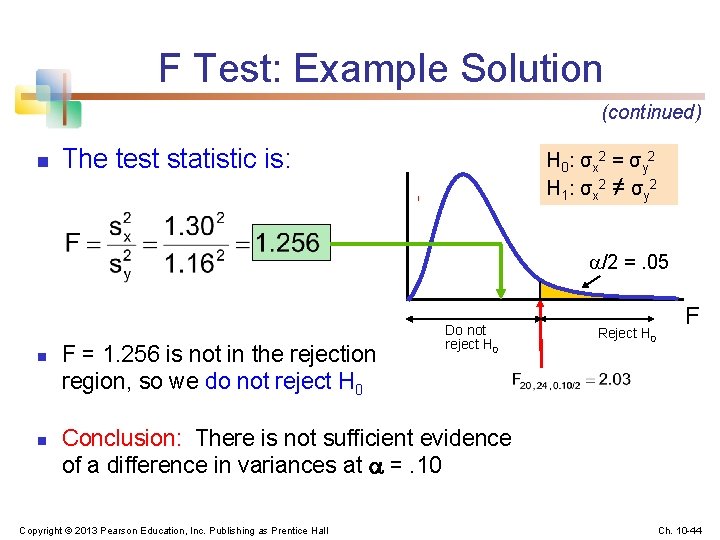
F Test: Example Solution (continued) n The test statistic is: H 0 : σx 2 = σy 2 H 1 : σx 2 ≠ σy 2 /2 =. 05 n n F = 1. 256 is not in the rejection region, so we do not reject H 0 Do not reject H 0 Reject H 0 F Conclusion: There is not sufficient evidence of a difference in variances at =. 10 Copyright © 2013 Pearson Education, Inc. Publishing as Prentice Hall Ch. 10 -44