MIS 331 Data Mining 20192020 Fall Chapter 7

MIS 331 Data Mining 2019/2020 Fall Chapter 7 -A Sampliing Distribution, Confidence Interval Estimation and Hypothesis Testing for Variance of a Population Copyright © 2013 Pearson Education, Inc. Publishing as Prentice Hall Ch. 6 -1

Outline n n n Sampling Distributio of Sample Variances Confidence Interval Estimation for the Variance Tests of the Variance of a Normal Distribution

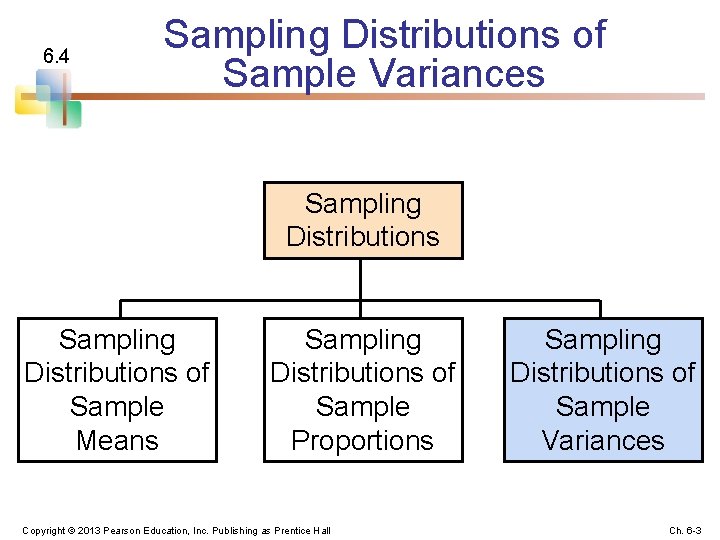
6. 4 Sampling Distributions of Sample Variances Sampling Distributions of Sample Means Sampling Distributions of Sample Proportions Copyright © 2013 Pearson Education, Inc. Publishing as Prentice Hall Sampling Distributions of Sample Variances Ch. 6 -3

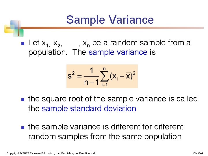
Sample Variance n n n Let x 1, x 2, . . . , xn be a random sample from a population. The sample variance is the square root of the sample variance is called the sample standard deviation the sample variance is different for different random samples from the same population Copyright © 2013 Pearson Education, Inc. Publishing as Prentice Hall Ch. 6 -4

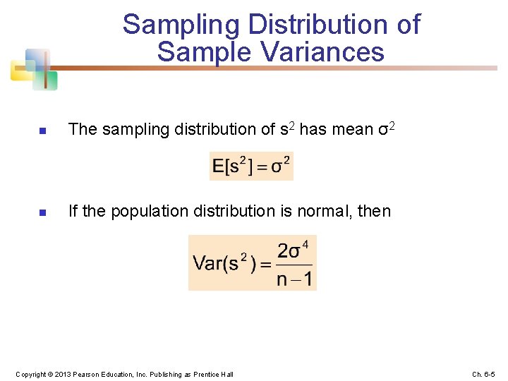
Sampling Distribution of Sample Variances n The sampling distribution of s 2 has mean σ2 n If the population distribution is normal, then Copyright © 2013 Pearson Education, Inc. Publishing as Prentice Hall Ch. 6 -5

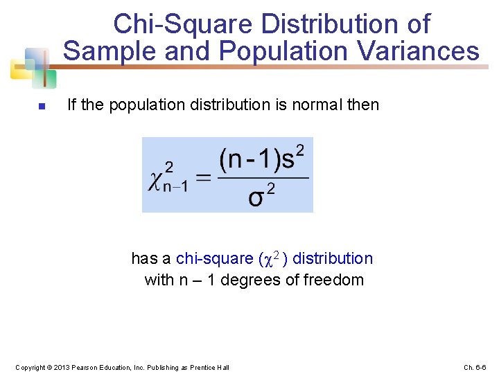
Chi-Square Distribution of Sample and Population Variances n If the population distribution is normal then has a chi-square ( 2 ) distribution with n – 1 degrees of freedom Copyright © 2013 Pearson Education, Inc. Publishing as Prentice Hall Ch. 6 -6

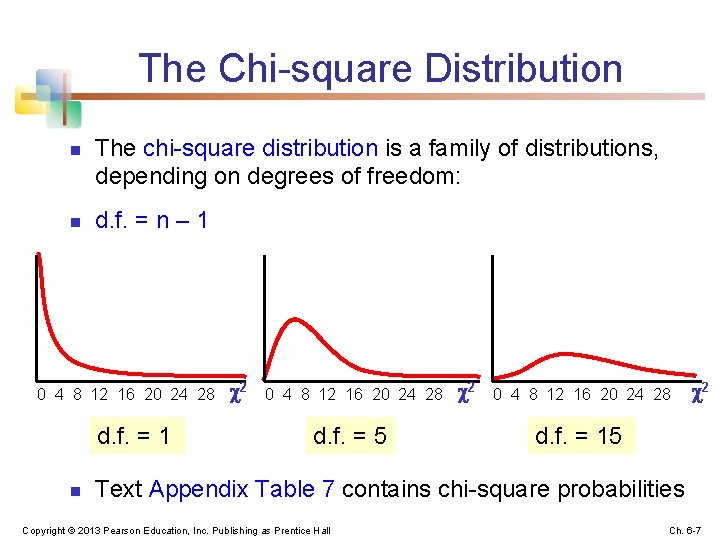
The Chi-square Distribution n n The chi-square distribution is a family of distributions, depending on degrees of freedom: d. f. = n – 1 0 4 8 12 16 20 24 28 d. f. = 1 n 2 0 4 8 12 16 20 24 28 d. f. = 5 2 0 4 8 12 16 20 24 28 2 d. f. = 15 Text Appendix Table 7 contains chi-square probabilities Copyright © 2013 Pearson Education, Inc. Publishing as Prentice Hall Ch. 6 -7

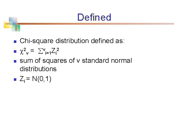
Defined n n Chi-square distribution defined as: 2 v = vi=1 Zi 2 sum of squares of v standard normal distributions Zi = N(0, 1)

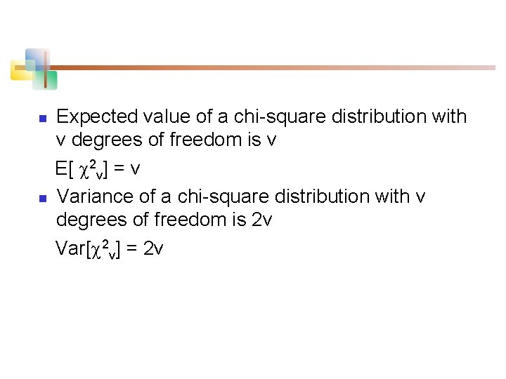
n n Expected value of a chi-square distribution with v degrees of freedom is v E[ 2 v] = v Variance of a chi-square distribution with v degrees of freedom is 2 v Var[ 2 v] = 2 v

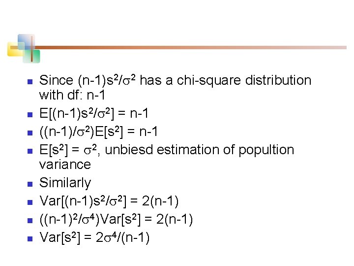
n n n n Since (n-1)s 2/ 2 has a chi-square distribution with df: n-1 E[(n-1)s 2/ 2] = n-1 ((n-1)/ 2)E[s 2] = n-1 E[s 2] = 2, unbiesd estimation of popultion variance Similarly Var[(n-1)s 2/ 2] = 2(n-1) ((n-1)2/ 4)Var[s 2] = 2(n-1) Var[s 2] = 2 4/(n-1)

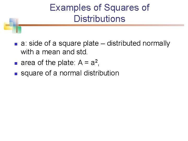
Examples of Squares of Distributions n n n a: side of a square plate – distributed normally with a mean and std. area of the plate: A = a 2, square of a normal distribution

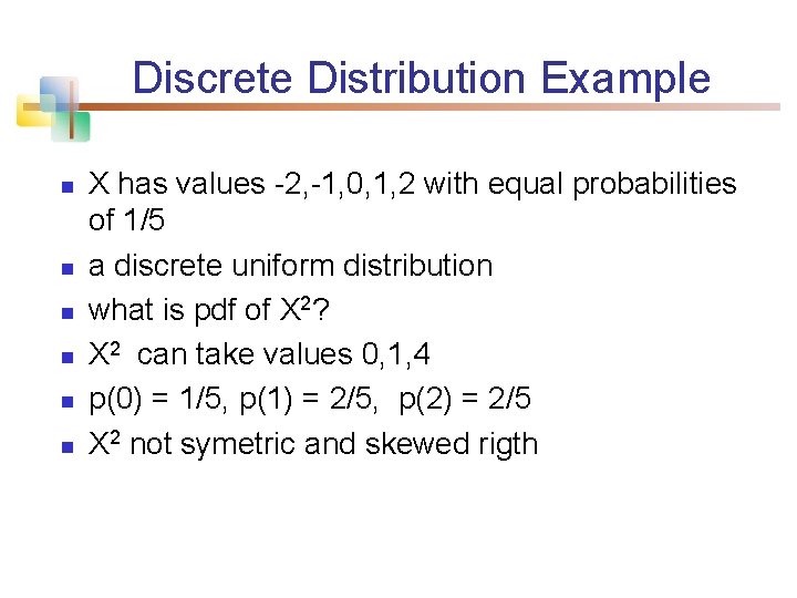
Discrete Distribution Example n n n X has values -2, -1, 0, 1, 2 with equal probabilities of 1/5 a discrete uniform distribution what is pdf of X 2? X 2 can take values 0, 1, 4 p(0) = 1/5, p(1) = 2/5, p(2) = 2/5 X 2 not symetric and skewed rigth

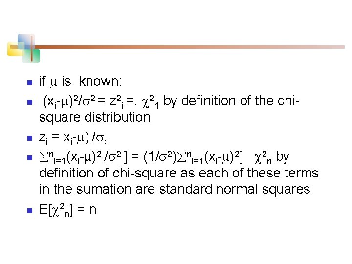
n n n E(xi- )2 = 2 definition of variance E[ ni=1(xi- )2] = n 2 expected value of n independent identical distributed (iid) random variables or E[ ni=1(xi- )2]/n = 2 unbiesd estimation of population variance when population mean is known

n n n if is known: (xi- )2/ 2 = z 2 i =. 21 by definition of the chisquare distribution zi = xi- ) / , ni=1(xi- )2 / 2 ] = (1/ 2) ni=1(xi- )2] 2 n by definition of chi-square as each of these terms in the sumation are standard normal squares E[ 2 n] = n

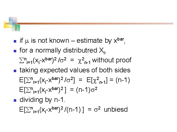
n n n if is not known – estimate by xbar, E[ ni=1(xi-xbar)2 ] = (n-1) 2 shown in Appandix of Chapter 6 of Newbold 8 independnet of distribution of Xi. sum of n quantities on the left makes only n-1 2. whan mean of the distribution is etimated by xbar

Exercise n n n Show with n = 2 E[ 2 i=1(xi-xbar)2 ] = 2 where xbar = (x 1+x 2)/2

n n if is not known – estimate by xbar, for a normally distributred Xi, ni=1(xi-xbar)2 / 2 = 2 n-1 without proof taking expected values of both sides E[ ni=1(xi-xbar)2 / 2] = E[ 2 n-1] = (n-1) E[ ni=1(xi-xbar)2 ] = (n-1) 2 dividing by n-1. E[ ni=1(xi-xbar)2 /(n-1) ] = 2 unbiesd

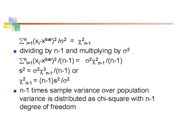
n n ni=1(xi-xbar)2 / 2 = 2 n-1 dividing by n-1 and multiplying by 2 ni=1(xi-xbar)2 /(n-1) = 2 2 n-1 /(n-1) s 2 = 2 2 n-1 /(n-1) or 2 n-1 = (n-1)s 2 / 2 n-1 times sample variance over population variance is distributed as chi-square with n-1 degree of freedom

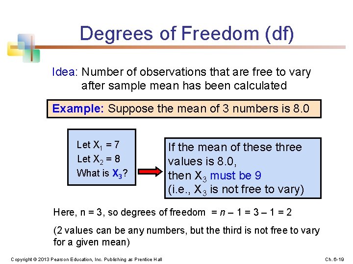
Degrees of Freedom (df) Idea: Number of observations that are free to vary after sample mean has been calculated Example: Suppose the mean of 3 numbers is 8. 0 Let X 1 = 7 Let X 2 = 8 What is X 3? If the mean of these three values is 8. 0, then X 3 must be 9 (i. e. , X 3 is not free to vary) Here, n = 3, so degrees of freedom = n – 1 = 3 – 1 = 2 (2 values can be any numbers, but the third is not free to vary for a given mean) Copyright © 2013 Pearson Education, Inc. Publishing as Prentice Hall Ch. 6 -19

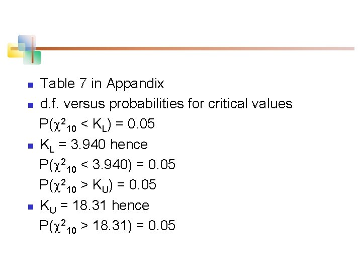
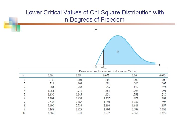
n n Table 7 in Appandix d. f. versus probabilities for critical values P( 210 < KL) = 0. 05 KL = 3. 940 hence P( 210 < 3. 940) = 0. 05 P( 210 > KU) = 0. 05 KU = 18. 31 hence P( 210 > 18. 31) = 0. 05

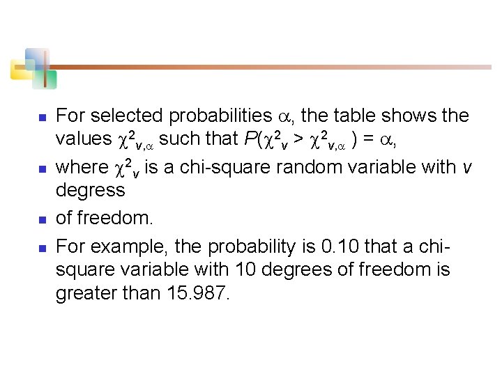
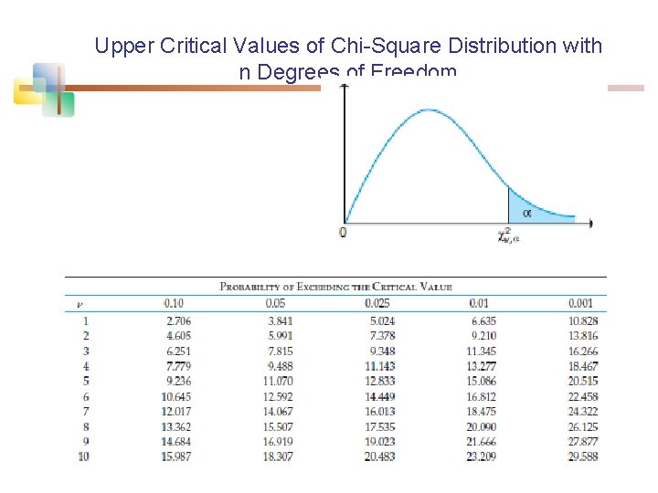
n n For selected probabilities , the table shows the values 2 v, such that P( 2 v > 2 v, ) = , where 2 v is a chi-square random variable with v degress of freedom. For example, the probability is 0. 10 that a chisquare variable with 10 degrees of freedom is greater than 15. 987.

Upper Critical Values of Chi-Square Distribution with n Degrees of Freedom

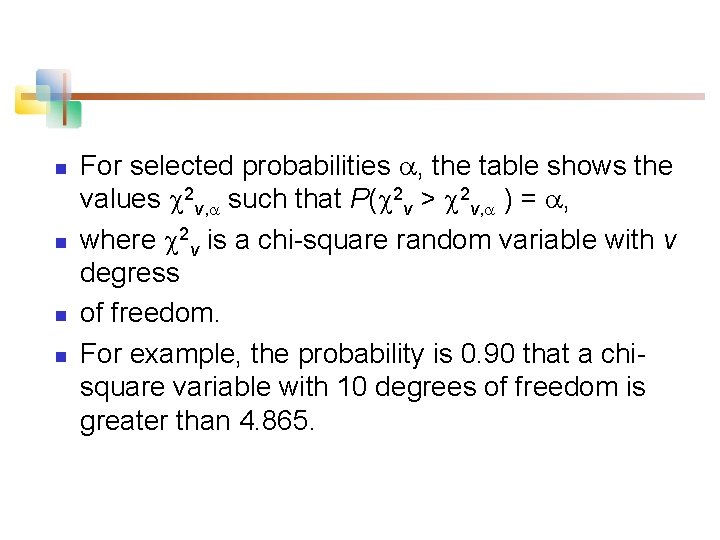
n n For selected probabilities , the table shows the values 2 v, such that P( 2 v > 2 v, ) = , where 2 v is a chi-square random variable with v degress of freedom. For example, the probability is 0. 90 that a chisquare variable with 10 degrees of freedom is greater than 4. 865.

Lower Critical Values of Chi-Square Distribution with n Degrees of Freedom

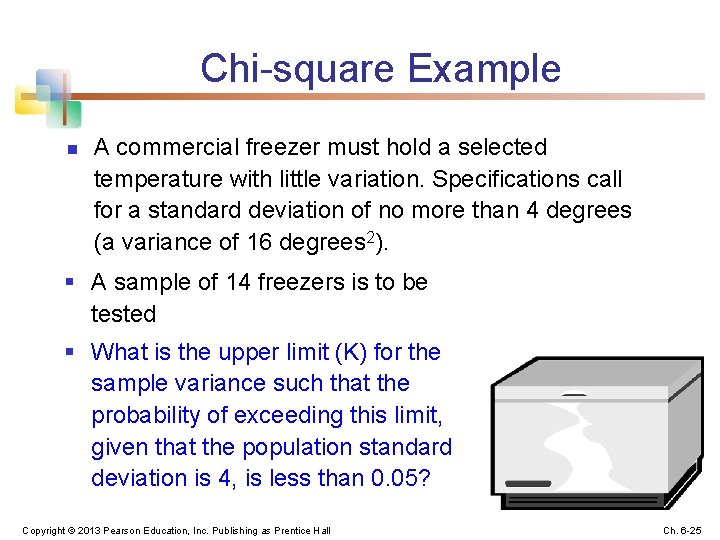
Chi-square Example n A commercial freezer must hold a selected temperature with little variation. Specifications call for a standard deviation of no more than 4 degrees (a variance of 16 degrees 2). § A sample of 14 freezers is to be tested § What is the upper limit (K) for the sample variance such that the probability of exceeding this limit, given that the population standard deviation is 4, is less than 0. 05? Copyright © 2013 Pearson Education, Inc. Publishing as Prentice Hall Ch. 6 -25

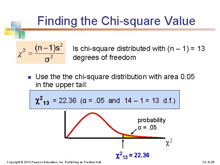
Finding the Chi-square Value Is chi-square distributed with (n – 1) = 13 degrees of freedom n Use the chi-square distribution with area 0. 05 in the upper tail: 213 = 22. 36 (α =. 05 and 14 – 1 = 13 d. f. ) probability α =. 05 2 213 = 22. 36 Copyright © 2013 Pearson Education, Inc. Publishing as Prentice Hall Ch. 6 -26

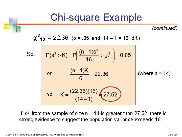
Chi-square Example (continued) 213 = 22. 36 (α =. 05 and 14 – 1 = 13 d. f. ) So: or (where n = 14) so If s 2 from the sample of size n = 14 is greater than 27. 52, there is strong evidence to suggest the population variance exceeds 16. Copyright © 2013 Pearson Education, Inc. Publishing as Prentice Hall Ch. 6 -27

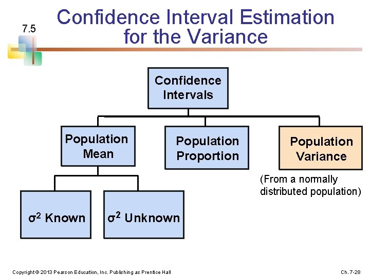
7. 5 Confidence Interval Estimation for the Variance Confidence Intervals Population Mean Population Proportion Population Variance (From a normally distributed population) σ2 Known σ2 Unknown Copyright © 2013 Pearson Education, Inc. Publishing as Prentice Hall Ch. 7 -28

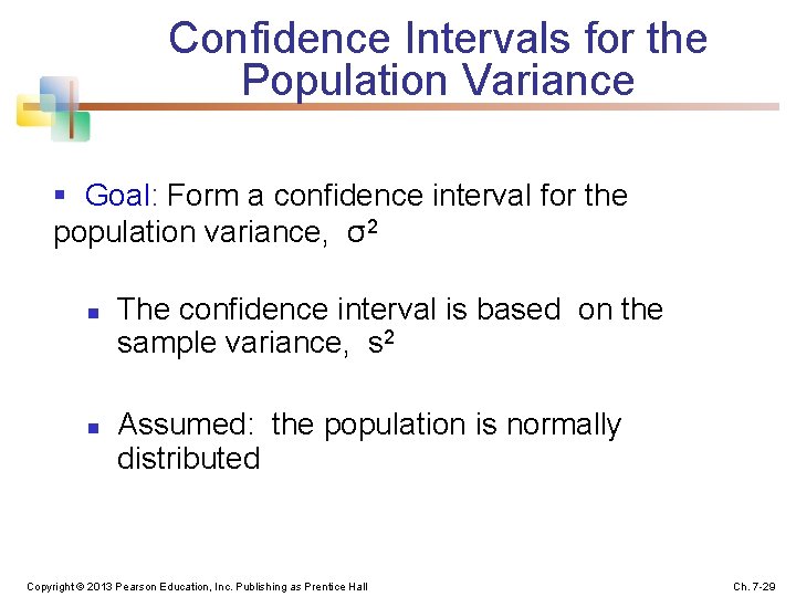
Confidence Intervals for the Population Variance § Goal: Form a confidence interval for the population variance, σ2 n n The confidence interval is based on the sample variance, s 2 Assumed: the population is normally distributed Copyright © 2013 Pearson Education, Inc. Publishing as Prentice Hall Ch. 7 -29

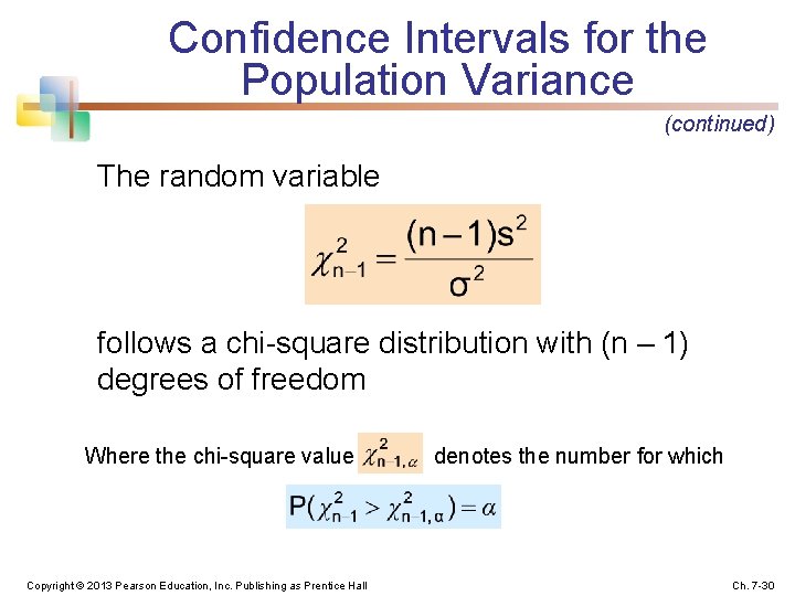
Confidence Intervals for the Population Variance (continued) The random variable follows a chi-square distribution with (n – 1) degrees of freedom Where the chi-square value Copyright © 2013 Pearson Education, Inc. Publishing as Prentice Hall denotes the number for which Ch. 7 -30

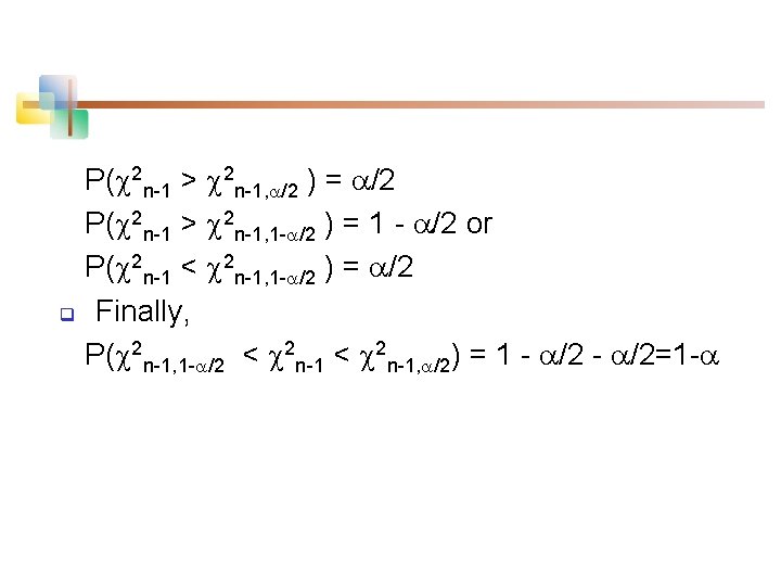
P( 2 n-1 > 2 n-1, /2 ) = /2 P( 2 n-1 > 2 n-1, 1 - /2 ) = 1 - /2 or P( 2 n-1 < 2 n-1, 1 - /2 ) = /2 q Finally, P( 2 n-1, 1 - /2 < 2 n-1, /2) = 1 - /2=1 -

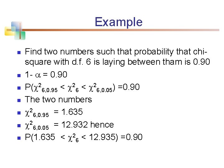
Example n n n n Find two numbers such that probability that chisquare with d. f. 6 is laying between tham is 0. 90 1 - = 0. 90 P( 26, 0. 95 < 26, 0. 05) =0. 90 The two numbers 26, 0. 95 = 1. 635 26, 0. 05 = 12. 932 hence P(1. 635 < 26 < 12. 935) =0. 90

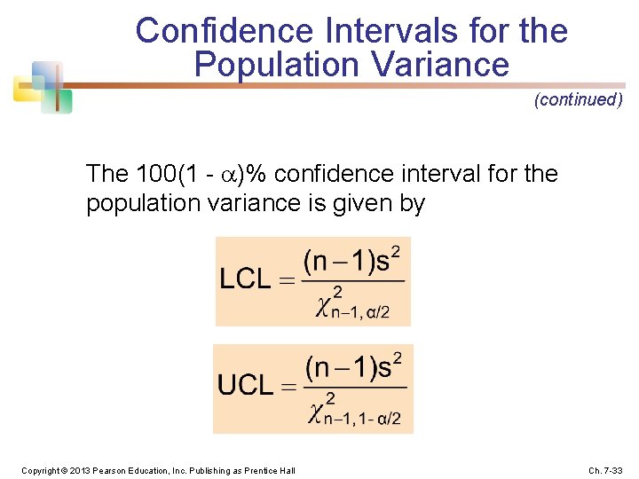
Confidence Intervals for the Population Variance (continued) The 100(1 - )% confidence interval for the population variance is given by Copyright © 2013 Pearson Education, Inc. Publishing as Prentice Hall Ch. 7 -33

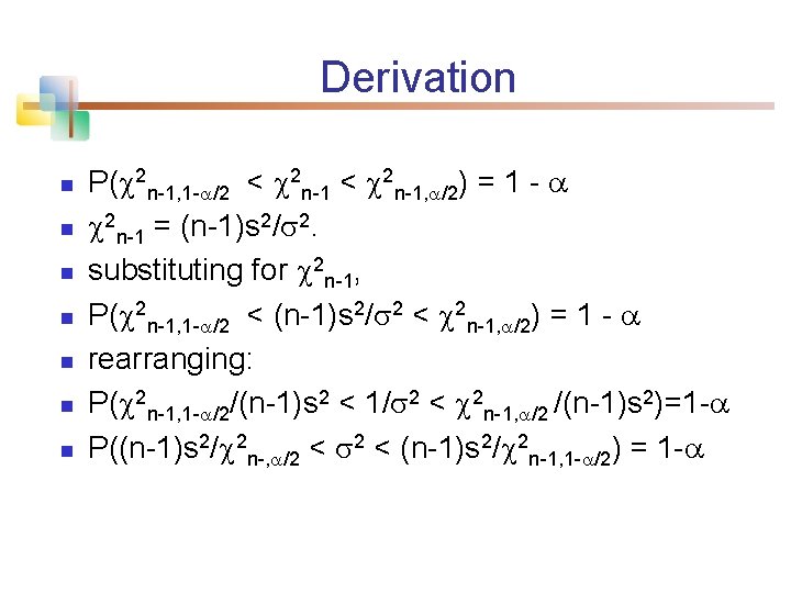
Derivation n n n P( 2 n-1, 1 - /2 < 2 n-1, /2) = 1 - 2 n-1 = (n-1)s 2/ 2. substituting for 2 n-1, P( 2 n-1, 1 - /2 < (n-1)s 2/ 2 < 2 n-1, /2) = 1 - rearranging: P( 2 n-1, 1 - /2/(n-1)s 2 < 1/ 2 < 2 n-1, /2 /(n-1)s 2)=1 - P((n-1)s 2/ 2 n-, /2 < (n-1)s 2/ 2 n-1, 1 - /2) = 1 -

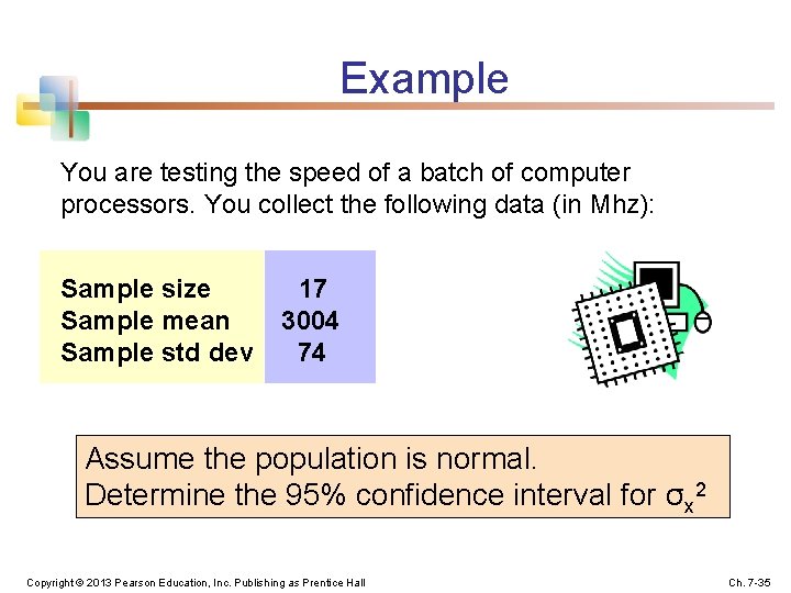
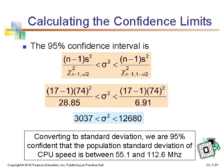
Example You are testing the speed of a batch of computer processors. You collect the following data (in Mhz): Sample size Sample mean Sample std dev 17 3004 74 Assume the population is normal. Determine the 95% confidence interval for σx 2 Copyright © 2013 Pearson Education, Inc. Publishing as Prentice Hall Ch. 7 -35

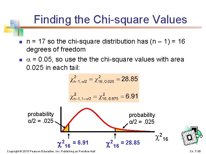
Finding the Chi-square Values n n n = 17 so the chi-square distribution has (n – 1) = 16 degrees of freedom = 0. 05, so use the chi-square values with area 0. 025 in each tail: probability α/2 =. 025 216 = 6. 91 Copyright © 2013 Pearson Education, Inc. Publishing as Prentice Hall 216 = 28. 85 216 Ch. 7 -36

Calculating the Confidence Limits n The 95% confidence interval is Converting to standard deviation, we are 95% confident that the population standard deviation of CPU speed is between 55. 1 and 112. 6 Mhz Copyright © 2013 Pearson Education, Inc. Publishing as Prentice Hall Ch. 7 -37

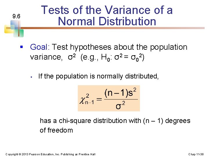
Tests of the Variance of a Normal Distribution 9. 6 § Goal: Test hypotheses about the population variance, σ2 (e. g. , H 0: σ2 = σ02) § If the population is normally distributed, has a chi-square distribution with (n – 1) degrees of freedom Copyright © 2013 Pearson Education, Inc. Publishing as Prentice Hall Chap 11 -38

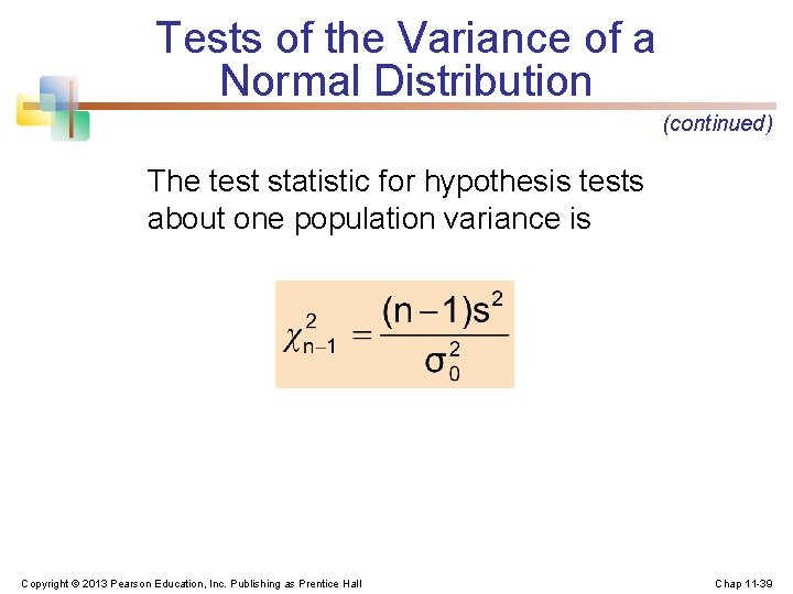
Tests of the Variance of a Normal Distribution (continued) The test statistic for hypothesis tests about one population variance is Copyright © 2013 Pearson Education, Inc. Publishing as Prentice Hall Chap 11 -39

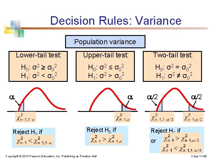
Decision Rules: Variance Population variance Lower-tail test: Upper-tail test: Two-tail test: H 0: σ 2 σ 02 H 1: σ 2 < σ 02 H 0: σ 2 ≤ σ 02 H 1: σ 2 > σ 02 H 0: σ 2 = σ 02 H 1: σ 2 ≠ σ 02 a Reject H 0 if a/2 Reject H 0 if or Copyright © 2013 Pearson Education, Inc. Publishing as Prentice Hall Chap 11 -40

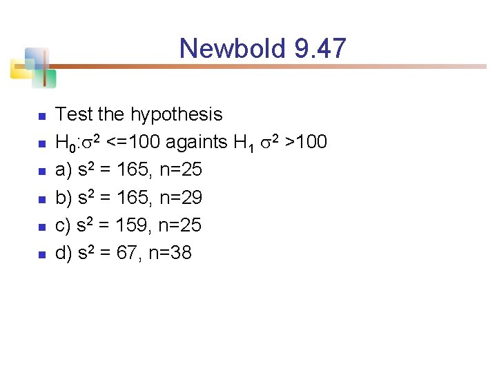
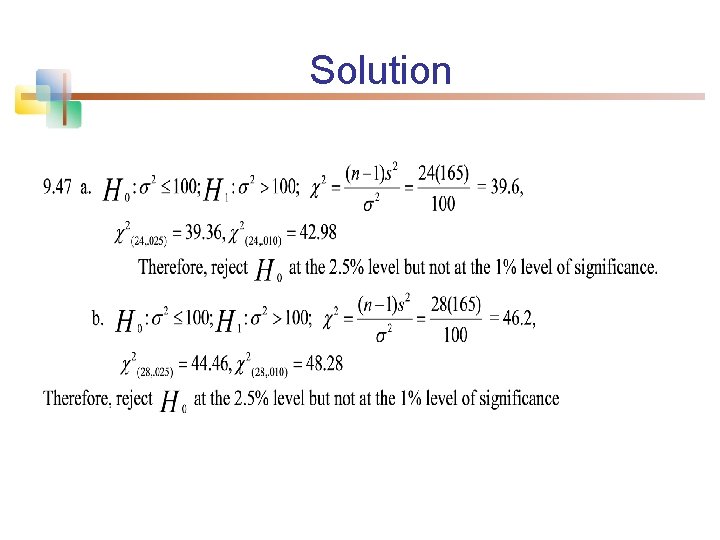
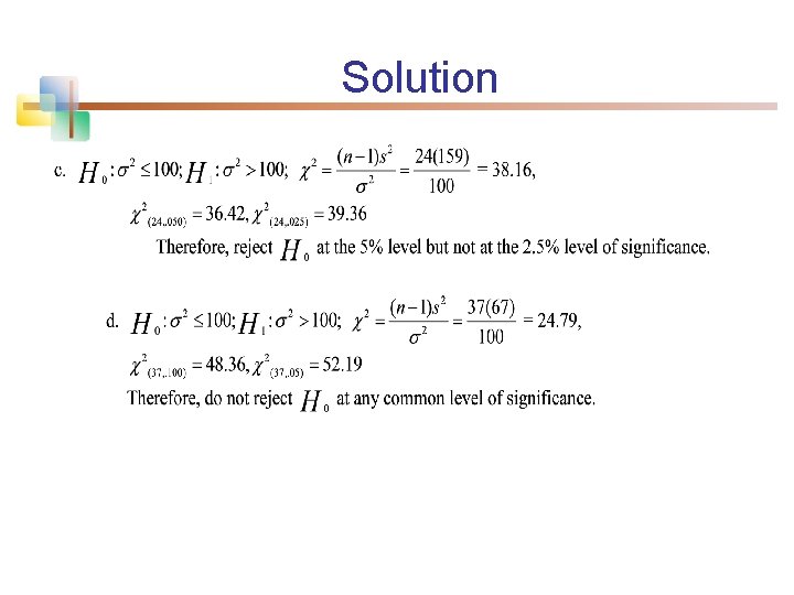
Newbold 9. 47 n n n Test the hypothesis H 0: 2 <=100 againts H 1 2 >100 a) s 2 = 165, n=25 b) s 2 = 165, n=29 c) s 2 = 159, n=25 d) s 2 = 67, n=38

Solution

Solution

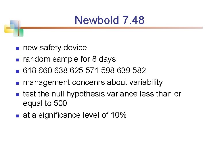
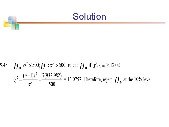
Newbold 7. 48 n n n new safety device random sample for 8 days 618 660 638 625 571 598 639 582 management concenrs about variability test the null hypothesis variance less than or equal to 500 at a significance level of 10%

Solution