Regression II w simple linear regression beta slope

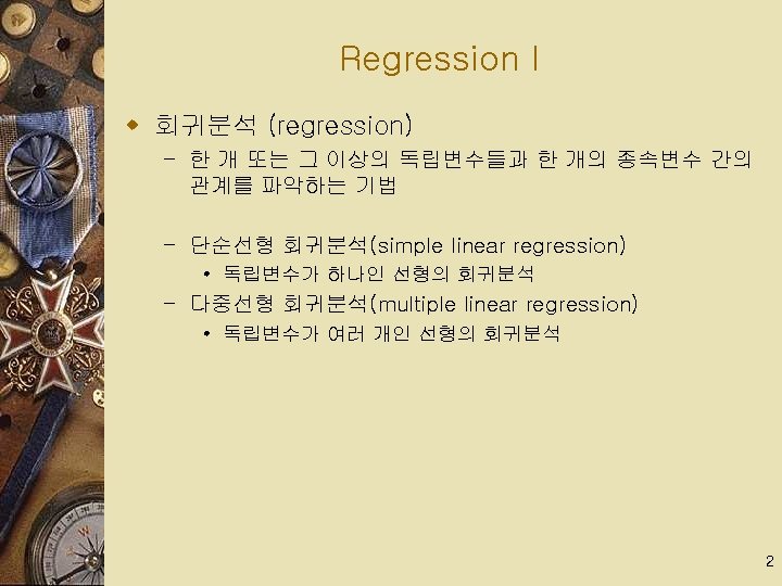
 – 단순선형 회귀분석의 회귀계수(β, beta)는 기울기(slope)를 의미함")
Regression II w 단순선형 회귀분석(simple linear regression) – 단순선형 회귀분석의 회귀계수(β, beta)는 기울기(slope)를 의미함 – 상관계수(Pearson r)는 예측의 정확성(prediction accuracy)을 의미함 y y x x 낮은 정의 상관관계 (low positive correlation) 높은 정의 상관관계 (high positive correlation) 3
는 기울기(slope) β = ∑i=1 n (xi -")
Regression III – 단순선형 회귀분석의 회귀계수(β, beta)는 기울기(slope) β = ∑i=1 n (xi - x )(yi - y ) ∑i=1 n (xi - x )2 – 상관계수(Pearson r)는 예측의 정확성(prediction accuracy) Cov(x, y) Sxy rxy = = Sx Sy STD(x) * STD(y) = ∑i=1 n (xi - x )(yi - y ) √ ∑i=1 n (xi - x)2 √ ∑i=1 n (yi - y)2 4
 w OLS Assumptions – Yi =")
Regression V w OLS (ordinary least square; 최소자승법) w OLS Assumptions – Yi = β 0 + β 1 Xi + εi – X와 Y는 선형종속관계이다 – 설명변수 X는 비확률변수이다 – εi ~ N(μi , σi 2) – E(εi) = μi = 0 – Var(εi) = σi 2 = σ2 [homoskedasticity] [Heteroskedasticity] – Cov(εi, εj) = 0 (for i ≠ j) [Independent error term] [Autocorrelation] 6
 – SPSS, 기술통계량-데이터 탐색 • Shapiro-Wilk Test or")
Regression VI w Normality (잔차 정규성) – SPSS, 기술통계량-데이터 탐색 • Shapiro-Wilk Test or Kolmogorov-Smirnov Test • 특히, 표본 수가 작을 때 • H 0 : normal – Graphical Methods • 표본 수가 크면 정규성 기각이 잘 됨 • e. g. Q-Q Plot (quantile-quantile plot) 7
 – Heteroskedasticity does not cause OLS coefficient estimates to")
Regression VII w Heteroskedasticity (이분산성) – Heteroskedasticity does not cause OLS coefficient estimates to be biased. However, the variance of the coefficients tends to be underestimated, inflating tscores and sometimes making insignificant variables appear to be statistically significant. – SAS, 근사 공분산행렬 – SAS, 동분산성에 대한 Chi-square test – H 0 : Homoskedasticity 8
 – Durbin-Watson Statistic ≒ 2 * (1 -ρ),")
Regression VIII w Autocorrelation (잔차들간의 상관계수) – Durbin-Watson Statistic ≒ 2 * (1 -ρ), -1 < ρ < 1 – While it does not bias the OLS coefficient estimates, the standard errors tend to be underestimated (and the tscores overestimated) when the autocorrelations of the errors at low lags are positive • H 0 : No Autocorrelation – 0 < DW < 4 • dl, du는 통계표가 따로 있음 (Savin and White, 1977) 4 -dl < DW < 4 : 음(-)의 연속상관 4 -du < DW < 4 -dl : 해석하기 힘듦 2 < DW < 4 -du : 연속상관 없음 (0) du < DW < 2 : 연속상관 없음 (0) dl < DW < du : 해석하기 힘듦 0 < DW < dl : 양(+)의 연속상관 9
 – A statistical problem that arises when")
Regression IX w Multicollinearity (독립변수간 높은 상관계수) – A statistical problem that arises when correlations between independent variables are extremely high, producing large standard errors of regression coefficients (beta, β) and unstable coefficients (Venkatraman, 1989). (1) Variance Inflation => Low t-value c. f. T-value = [ β – hypothesized β ] / s. e. (β) (2) Large p-value of β (3) can not reject H 0: β=0 – 전형적인 현상 • 높은 상관계수의 변수들 다수: 여러 독립변수 중 특정 독립변 수만 유의 • 회귀계수의 불안정성 10

Regression X – Multicollinearity를 확인하는 네 가지 지표 • • Tolerance, 0. 1 이하 Variance Inflation Factor (VIF), 10 이상 Eigenvalue, 0. 01 이하 Condition Index, 100 이상 – 해결방안 • 여러 독립변수들 중에서 일부 제거 • 표본의 추가 확보 • 경우에 따라 평균변환변수(mean-centered variable) 사용 11

Control Variable w Concept of control variable – – Predictor of Dependent Variable But, No interest in this study Show distinctively the impact of independent variables e. g. 친절과 만족도 연구, 인테리어의 수준을 통제 w In statistical term – Yi = b 0 + bs CVsi + ei – Yi = b 0 + bs CVsi + b 1 Xi + b 2 Zi + ei – No interpretation on CVs 12
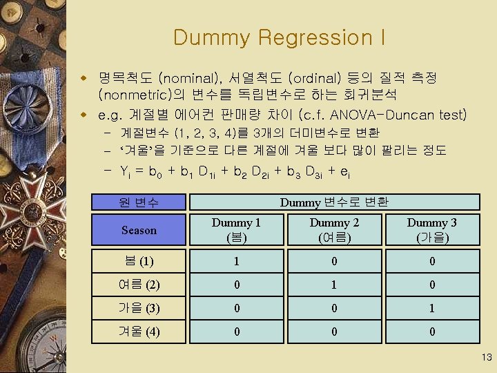

Quadratic Regression I w 2차 방정식: Y = a x 2 + b x + c a >0 Y a =0 a <0 - b/2 a X 15

Quadratic Regression II w 2차 방정식: Y = a x 2 + b x + c a >0, b>0 Y a >0, b<0 a =0, b>0 a =0, b<0 a <0, b>0 0 X 16

Quadratic Regression III w Yi = b 0 + b 1 xi + b 2 xi 2 + ei w b 2 = 0, Linear relationship – b 1 > 0, Positive relationship – b 1 < 0, Negative relationship – b 1 = 0, No relationship w b 2 > 0, – b 1 < 0, U-shaped relationship – b 1 0, xi >0인 영역에서 positive relationship과 유사 w b 2 < 0, – b 1 > 0, Reverse U-shaped relationship – b 1 ≤ 0, xi >0인 영역에서 negative relationship과 유사 17

Quadratic Regression IV w Model Comparison – Original model • Yi = b 0 + b 1 Xi + b 2 Xi 2 + ei – Mean-centered model • Let mc. Xi = Xi – X • [ New Model ] • Yi = mcb 0 + mcb 1 mc. Xi + mcb 2 mc. Xi 2 + mcei • Yi = b 0 + b 1 Xi + b 2 Xi 2 + ei [ Original Model ] • Yi = b 0 + b 1 (mc. Xi+ X ) + b 2 (mc. Xi+ X )2 + ei • Yi = b 0+b 1 X+b 2 X 2 + (b 1+2 b 2 X)mc. Xi + b 2 mc. Xi 2 + ei • i. e. mcb 0 = b 0+b 1 X+b 2 X 2 ; mcb 1 = b 1+2 b 2 X ; mcb 2 = b 2 18

Quadratic Regression V w Yi = mcb 0 + mcb 1 xi + mcb 2 xi 2 + mcei w mcb 2 = 0, Linear relationship – mcb 1 > 0, Positive relationship – mcb 1 < 0, Negative relationship – mcb 1 = 0, No relationship w mcb 2 > 0, – mcb 1 ≤ 0, U-shaped relationship – mcb 1 > 0, U-shaped or positive relationship w mcb 2 < 0, – mcb 1 ≥ 0, Reverse U-shaped relationship – mcb 1 < 0, reverse U-shaped or positive relationship w <SP-5 EE_data. xls>로 실습 19

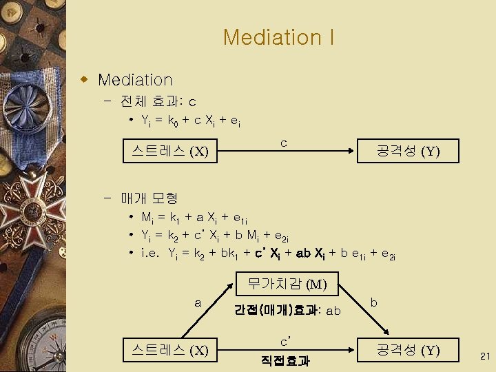
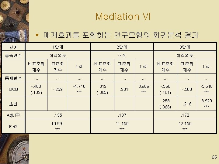
 – c = c’ + ab")
Mediation II w 전체효과 = 직접효과 + 간접효과(매개효과) – c = c’ + ab w 매개효과의 존재 – ab : significant – 완전 매개효과 (full mediation) • & c’ : not significant – 부분 매개효과 (partial mediation) • & c’ : significant 22
 27")
Mediation VII w 심덕섭·양동민·하성욱 (2010) 27

Mediation VIII 28

 variable has on a criterion")
Moderation I w The impact that a predictor (independent) variable has on a criterion (dependent) variable is dependent on the level of a third variable (moderator). – Criterion-specific: Fit definition means the influence to Y – Interaction term: Independent * Moderator – Moderated Regression Analysis • Yi = b 0 + b 1 Xi + b 2 Zi + b 3 Xi*Zi + ei • Yi = b 0 + (b 1 + b 3 Zi )*Xi + b 2 Zi + ei w Research Model Appearance of Employees (Z) Independent Kindness of Employees (X) Moderator b 2 b 3 Zi b 1 Dependent Sales Volume of Store (Y) 31

Moderation II w 연구결과의 예 Sales Appearance: H Appearance: M Appearance: L Kindness 32

Moderation III : Mean-centering I w Not raw score, But the mean-centered score of each variable (Venkatraman, 1989) – Mean-centering (평균 중심화) • mc. Xi = Xi – X • mc. Zi = Zi – Z – Multicollinearity issue (다중공선성) • With X and Z bivariate normal, Corr (mc. Xmc. Z, mc. X) = 0 – Interpretation issue • • • Yi = b 0 + b 1 Xi + b 2 Zi + b 3 Xi*Zi + ei Yi = b 0 + (b 1 + b 3 Zi )*Xi + b 2 Zi + ei b 1 means the impact of X on Y when Z=0 b 2 means the impact of Z on Y when X=0 If Z doesn’t have zero value, b 1 doesn’t have meaning. If X doesn’t have zero value, b 2 doesn’t have meaning. • mcb 1 means the impact of X on Y when Z= Z • mcb 2 means the impact of Z on Y when X= X 33

Moderation IV : Mean-centering II w Model Comparison – Original model • Yi = b 0 + b 1 Xi + b 2 Zi + b 3 Xi*Zi + ei • Yi = b 0 + (b 1 + b 3 Zi )*Xi + b 2 Zi + ei – Mean-centered model • • Let mc. Xi = Xi – X Let mc. Zi = Zi – Z [ New Model ] Yi = mcb 1 mc. Xi + mcb 2 mc. Zi + mcb 3 mc. Xi*mc. Zi + mcb 0 + mcei • Yi = b 1 Xi + b 2 Zi + b 3 Xi*Zi + b 0 + ei [ Original Model ] • Yi = b 1(mc. Xi+ X) + b 2(mc. Zi+ Z) + b 3(mc. Xi+ X)*(mc. Zi+ Z )+ b 0 + ei • Yi = (b 1+b 3 Z)*mc. Xi + (b 2+b 3 X)*mc. Zi + b 3 mc. Xi*mc. Zi + (b 0 + b 1 X+ b 2 Z+ b 3 X Z) + ei • i. e. mcb 1 = b 1+b 3 Z ; mcb 2 = b 2+b 3 X ; mcb 3 = b 3 34

Moderation VII Raw variables 비표준화계수 표준오차 상수 5. 252 . 272 Kindness . 224 . 032 Appearance . 102 t 유의확률 19. 289 . 000 . 167 7. 057 . 000 . 026 . 092 3. 893 . 000 비표준화계수 표준오차 표준화계수 t 유의확률 상수 6. 238 . 561 124. 859 . 000 Kindness -. 046 . 138 . 166 6. 984 . 000 Appearance -. 004 . 059 . 092 3. 892 . 000 . 029 . 014 . 048 2. 009 . 045 표준오차 표준화계수 t 유의확률 124. 859 . 000 Raw variables K*A 표준화계수 <SP-5 Moderation. sav> Mean-Centering 비표준화계수 상수 7. 015 . 056 mc_Kindness . 222 . 032 . 166 6. 984 . 000 mc_Appearance . 102 . 026 . 092 3. 892 . 000 mc_K*mc_A . 029 . 014 . 048 2. 009 . 045 37
 Sales Ŝ = 0. 284 K + 7.")
Moderation VIII w 단순회귀선(simple regression line) Sales Ŝ = 0. 284 K + 7. 233 Ŝ = 0. 222 K + 7. 015 Ŝ = 0. 160 K + 6. 796 <SP-5 EE_data. xls> Kindness 38
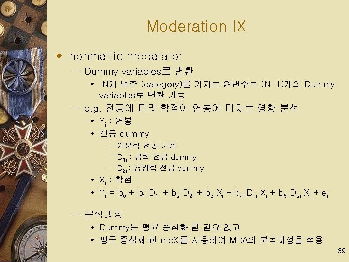

Moderation X : Subgroup Analysis w Nonmetric moderator or Alterative to MRA – Fisher’s Z-test (or T-statistic or Chi-squared statistic) – Z = ½ ln [ (1+r 1)/(1 -r 1) ] - ½ ln [ (1+r 2)/(1 -r 2) ] √ [ 1/(n 1 -1) + 1/(n 2 -1) ] – ni : i 그룹 표본수, ri : i 그룹 상관계수 Correlation b/w Kindness of Employees & Sales Volume of Store Low Appearance Group (n 1=24) High Appearance Group (n 2=18) Z-test 0. 316 0. 816 *** -2. 56 ** 주) + : p<0. 1; * : p<0. 05; ** : p<0. 01; *** : p<0. 001 40
")
Multicollinearity Issues w Mean Centering: – X 대신 mc. X [ i. e. X-mean(X) ]로 추정 – Reduction of correlation • With X and Z bivariate normal, Corr (mc. Xmc. Z, mc. X) = 0 w Fit regression: Moderation – X 대신 mc. X [ i. e. X-mean(X) ]로 추정 – Z 대신 mc. Z [ i. e. Z-mean(Z) ]로 추정 – X*Z 대신 mc. X*mc. Z [ i. e. (X-mean(X))*(Z-mean(Z)) ]로 추정 w Quadratic regression – X 대신 mc. X [ i. e. X-mean(X) ]로 추정 – X 2 대신 mc. X 2 [ i. e. (X-mean(X))2 ]로 추정 41

Matching I w The match between the one independent variable and the other independent variable – Match b/w Environment & Organizational Structure (Burns and Stalker, 1961) Negative Absolute Difference Uncertain Misfit Environmental Uncertainty Stable Fit Fit Misfit Mechanic NAD = 0 Organic Organizational Structure 42

Matching II w Criterion-Free: Fit definition is independent of Y w Negative absolute difference term: - | EU – OS | – Not raw score, But the standardized score of each variable (Bourgeois, 1985; Venkatraman, 1989) w Research Model Environmental Uncertainty b 1 b 3 Organizational Structure w Deviation Score Analysis Dependent Firm Performance b 2 <SP-5 EE_data. xls> – Performancei = b 0 + b 1 EUi + b 2 OSi - b 3 | EUi - OSi |+ ei 43

Fit effect w Concept of Fit – Contingency, Match, Consistency, Fit, Congruence, Coalignment (Venkatraman, 1989) Low Fit as profile deviation Fit as Gestalts Many (e. g. cluster analysis) Precise Functional Form High Fit as Mediation Fit as Covariation (e. g. factor analysis) Fit as Moderation Fit as Matching Criterion-specific Criterion-free Fitness anchoring a particular criterion (e. g. effectiveness) The # of Variables Involved Few 44
’s Strategy Type •")
Other Fit Concepts I w Gestalts – Miles and Snow (1978)’s Strategy Type • Prospectors, Analyzers, Defenders, Reactors – By Cluster Analysis • i. e. Distance between samples 45

Other Fit Concepts II w Profile Deviation – Deviation from Ideal Profile 46

Other Fit Concepts III w Covariation: Internal Consistency – Second-order, Confirmatory Factor Analysis 47

Questions w Regression – Simple linear regression, Multiple linear regression – OLS Assumptions: Normality, Heteroskedasticity, Autocorrelation, Multicollinearity – Control Variable – Dummy Regression – Quadratic Regression w Mediation – Baron & Kenny (1986), Sobel test w Moderation – Moderated regression analysis (MRA) – Nonmetric moderator, Subgroup analysis w Matching w Fit effect 48
- Slides: 48