Quantum Speedups for Semidefinite Programming Fernando G S

Quantum Speed-ups for Semidefinite Programming Fernando G. S. L. Brandão MSR -> Caltech based on joint work with Krysta Svore MSR Faculty Summit 2016

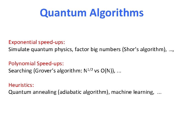
Quantum Algorithms Exponential speed-ups: Simulate quantum physics, factor big numbers (Shor’s algorithm), …, Polynomial Speed-ups: Searching (Grover’s algorithm: N 1/2 vs O(N)), . . . Heuristics: Quantum annealing (adiabatic algorithm), machine learning, . . .

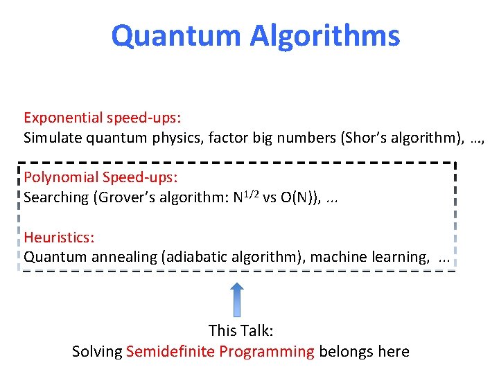
Quantum Algorithms Exponential speed-ups: Simulate quantum physics, factor big numbers (Shor’s algorithm), …, Polynomial Speed-ups: Searching (Grover’s algorithm: N 1/2 vs O(N)), . . . Heuristics: Quantum annealing (adiabatic algorithm), machine learning, . . . This Talk: Solving Semidefinite Programming belongs here

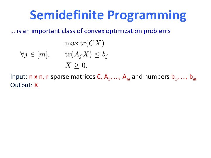
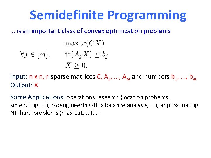
Semidefinite Programming … is an important class of convex optimization problems Input: n x n, r-sparse matrices C, A 1, . . . , Am and numbers b 1, . . . , bm Output: X Some Applications: operations research (location probems, scheduing, . . . ), bioengineering (flux balance analysis, . . . ), approximating NP-hard problems (max-cut, . . . ), field theory (conformal bootstraping), . . . Algorithms Interior points: Multilicative Weights: O((m 2 nr + mn 2)log(1/ε)) O((mnr/ε 2)) Lower bound: No faster than Ω(nm), for constant ε and r

Semidefinite Programming … is an important class of convex optimization problems Input: n x n, r-sparse matrices C, A 1, . . . , Am and numbers b 1, . . . , bm Output: X Some Applications: operations research (location probems, scheduling, . . . ), bioengineering (flux balance analysis, . . . ), approximating NP-hard problems (max-cut, . . . ), . . . Algorithms Interior points: Multilicative Weights: O((m 2 nr + mn 2)log(1/ε)) O((mnr/ε 2)) Lower bound: No faster than Ω(nm), for constant ε and r

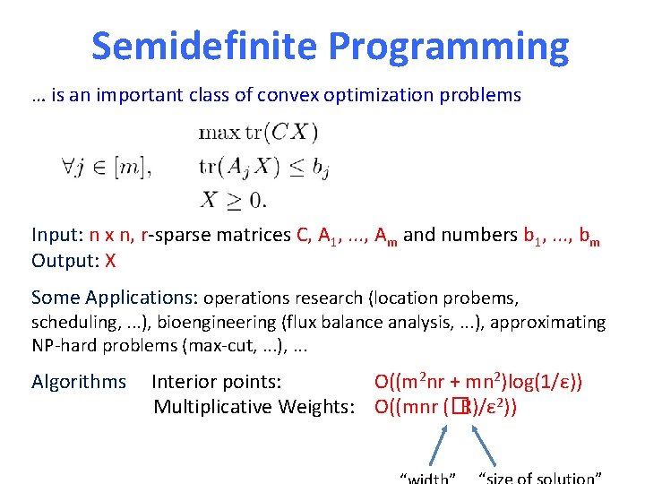
Semidefinite Programming … is an important class of convex optimization problems Input: n x n, r-sparse matrices C, A 1, . . . , Am and numbers b 1, . . . , bm Output: X Some Applications: operations research (location probems, scheduling, . . . ), bioengineering (flux balance analysis, . . . ), approximating NP-hard problems (max-cut, . . . ), . . . Algorithms Interior points: O((m 2 nr + mn 2)log(1/ε)) Multiplicative Weights: O((mnr (�R)/ε 2)) Lower bound: No faster than Ω(nm), for constant ε and r

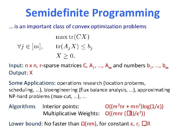
Semidefinite Programming … is an important class of convex optimization problems Input: n x n, r-sparse matrices C, A 1, . . . , Am and numbers b 1, . . . , bm Output: X Some Applications: operations research (location probems, scheduling, . . . ), bioengineering (flux balance analysis, . . . ), approximating NP-hard problems (max-cut, . . . ), . . . Algorithms Interior points: O((m 2 nr + mn 2)log(1/ε)) Multiplicative Weights: O((mnr (�R)/ε 2)) Lower bound: No faster than Ω(nm), for constant ε, r, �, R

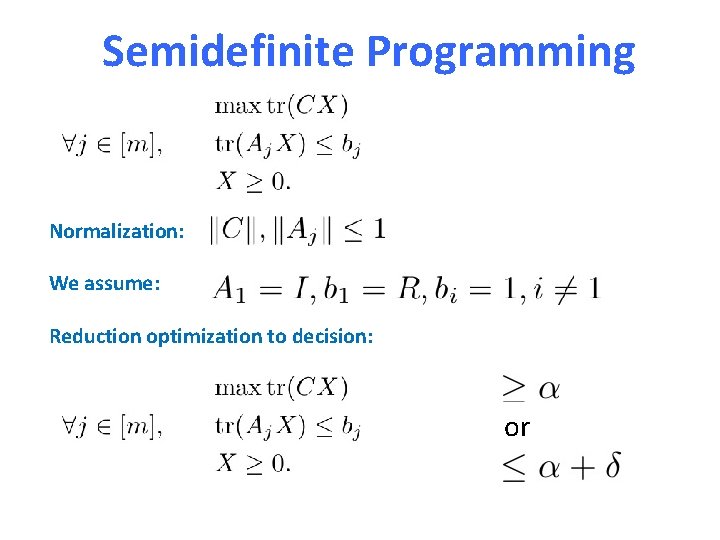
Semidefinite Programming Normalization: We assume: Reduction optimization to decision: or

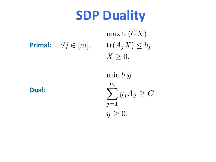
SDP Duality Primal: Dual:

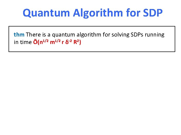
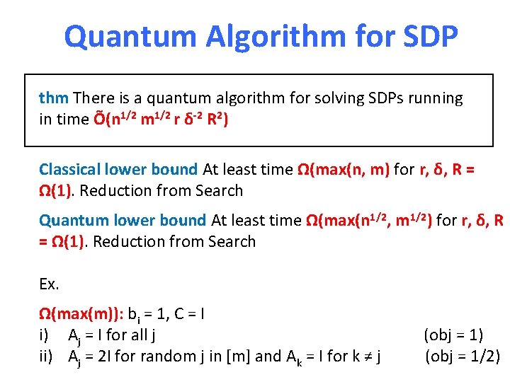
Quantum Algorithm for SDP thm There is a quantum algorithm for solving SDPs running in time Õ(n 1/2 m 1/2 r δ-2 R 2)

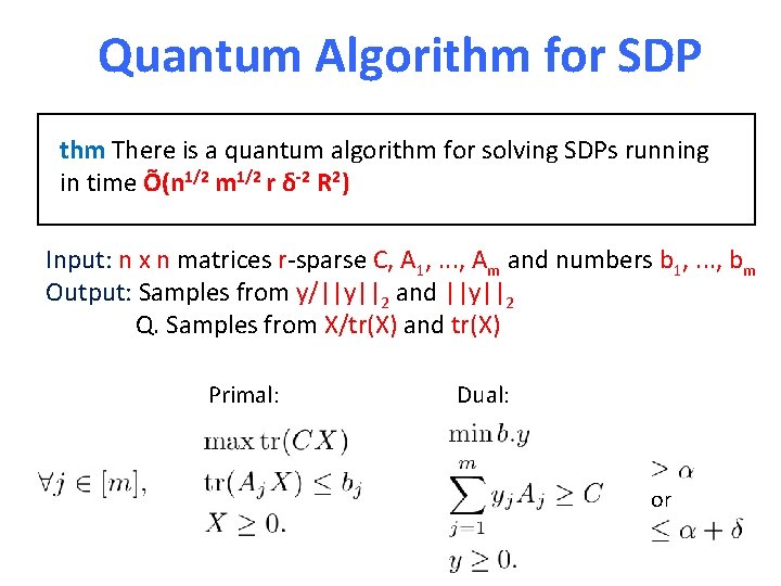
Quantum Algorithm for SDP thm There is a quantum algorithm for solving SDPs running in time Õ(n 1/2 m 1/2 r δ-2 R 2) Input: n x n matrices r-sparse C, A 1, . . . , Am and numbers b 1, . . . , bm Output: Samples from y/||y||2 and ||y||2 Q. Samples from X/tr(X) and tr(X) Primal: Dual: or

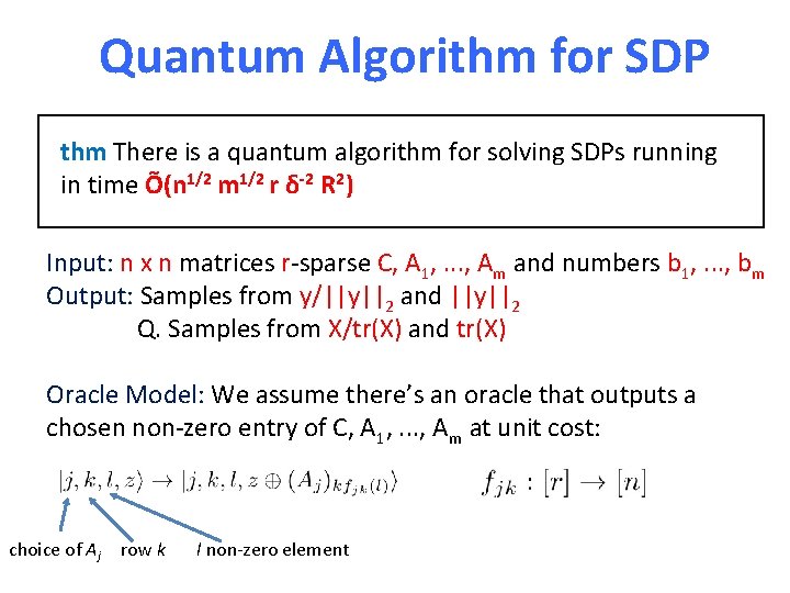
Quantum Algorithm for SDP thm There is a quantum algorithm for solving SDPs running in time Õ(n 1/2 m 1/2 r δ-2 R 2) Input: n x n matrices r-sparse C, A 1, . . . , Am and numbers b 1, . . . , bm Output: Samples from y/||y||2 and ||y||2 Q. Samples from X/tr(X) and tr(X) Oracle Model: We assume there’s an oracle that outputs a chosen non-zero entry of C, A 1, . . . , Am at unit cost: choice of Aj row k l non-zero element

Quantum Algorithm for SDP thm There is a quantum algorithm for solving SDPs running in time Õ(n 1/2 m 1/2 r δ-2 R 2) Classical lower bound At least time Ω(max(n, m) for r, δ, R = Ω(1). Reduction from Search Quantum lower bound At least time Ω(max(n 1/2, m 1/2) for r, δ, R = Ω(1). Reduction from Search Ex. Ω(max(m)): bi = 1, C = I i) Aj = I for all j ii) Aj = 2 I for random j in [m] and Ak = I for k ≠ j (obj = 1) (obj = 1/2)

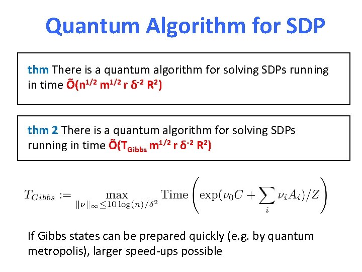
Quantum Algorithm for SDP thm There is a quantum algorithm for solving SDPs running in time Õ(n 1/2 m 1/2 r δ-2 R 2) thm 2 There is a quantum algorithm for solving SDPs running in time Õ(TGibbs m 1/2 r δ-2 R 2) If Gibbs states can be prepared quickly (e. g. by quantum metropolis), larger speed-ups possible

Quantum Algorithm for SDP The quantum algorithm is based on a classical algorithm for SDP due to Arora and Kale (2007) based on the multiplicative weight method Let’s review their method

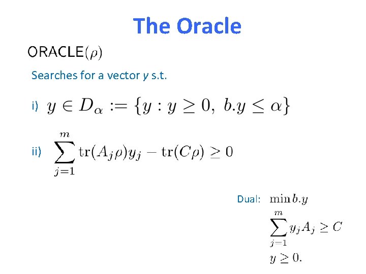
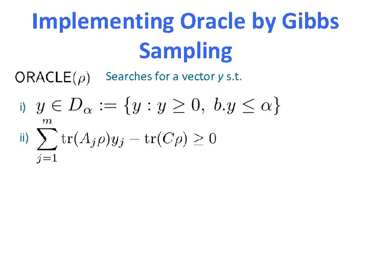
The Oracle Searches for a vector y s. t. i) ii) Dual:

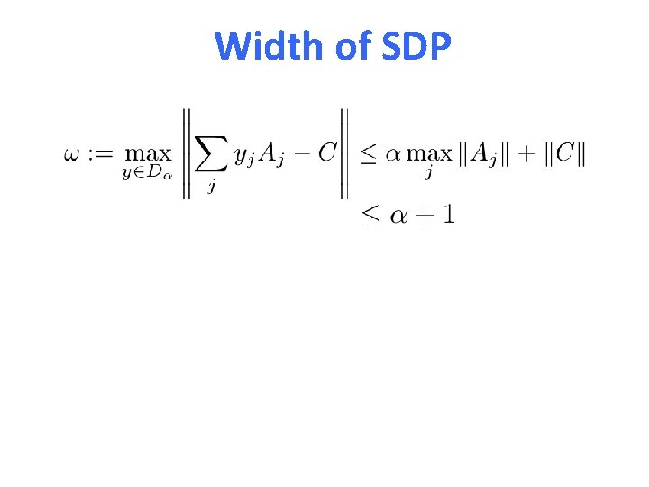
Width of SDP

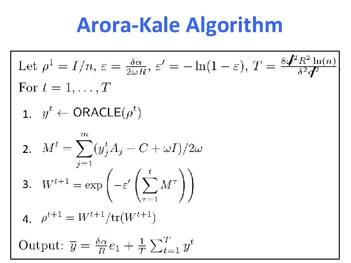
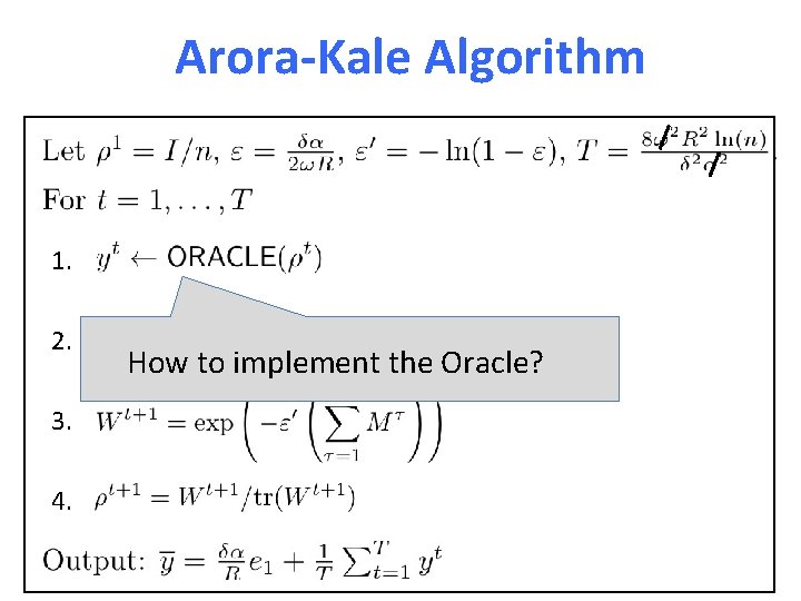
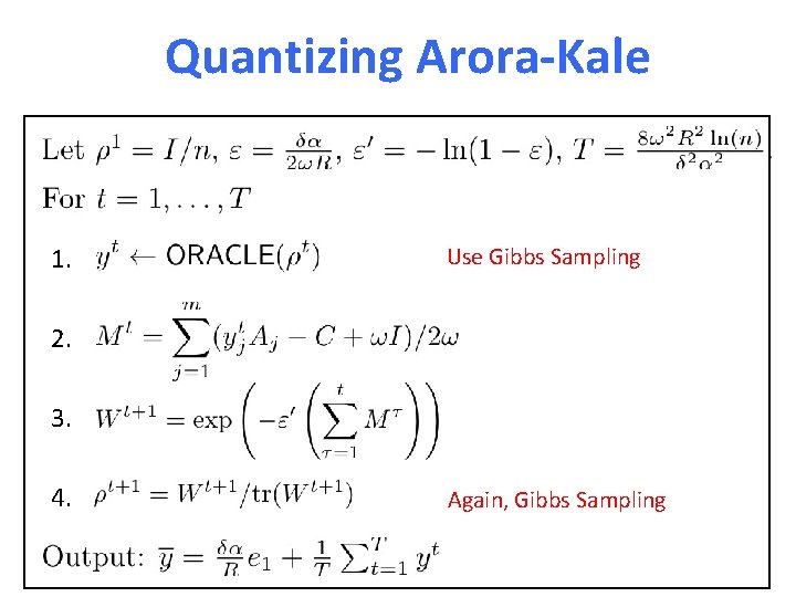
Arora-Kale Algorithm 1. 2. 3. 4.

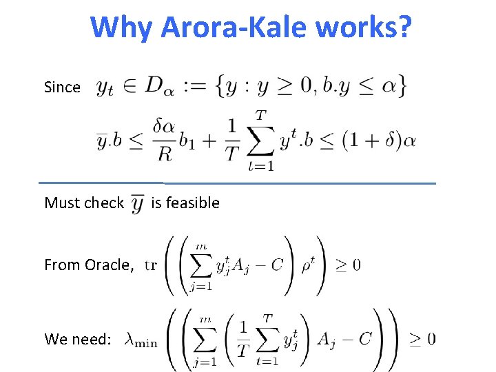
Why Arora-Kale works? Since Must check From Oracle, We need: is feasible

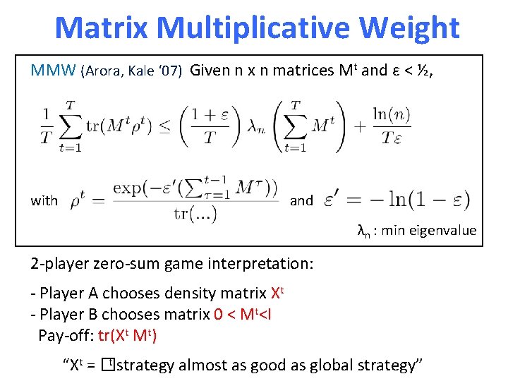
Matrix Multiplicative Weight MMW (Arora, Kale ‘ 07) Given n x n matrices Mt and ε < ½, with and λn : min eigenvalue 2 -player zero-sum game interpretation: - Player A chooses density matrix Xt - Player B chooses matrix 0 < Mt<I Pay-off: tr(Xt Mt) “Xt = �t strategy almost as good as global strategy”

Arora-Kale Algorithm 1. 2. 3. 4.

Arora-Kale Algorithm 1. 2. 3. 4. How to implement the Oracle?

Implementing Oracle by Gibbs Sampling Searches for a vector y s. t. i) ii)

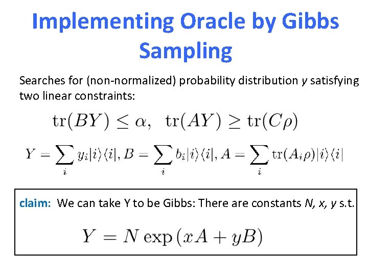
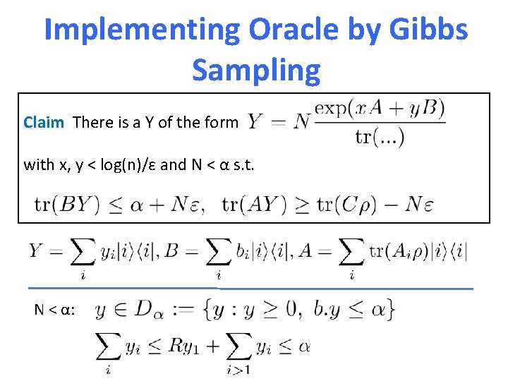
Implementing Oracle by Gibbs Sampling Searches for (non-normalized) probability distribution y satisfying two linear constraints: claim: We can take Y to be Gibbs: There are constants N, x, y s. t.

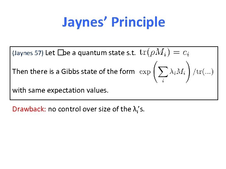
Jaynes’ Principle (Jaynes 57) Let �be a quantum state s. t. Then there is a Gibbs state of the form with same expectation values. Drawback: no control over size of the λi’s.

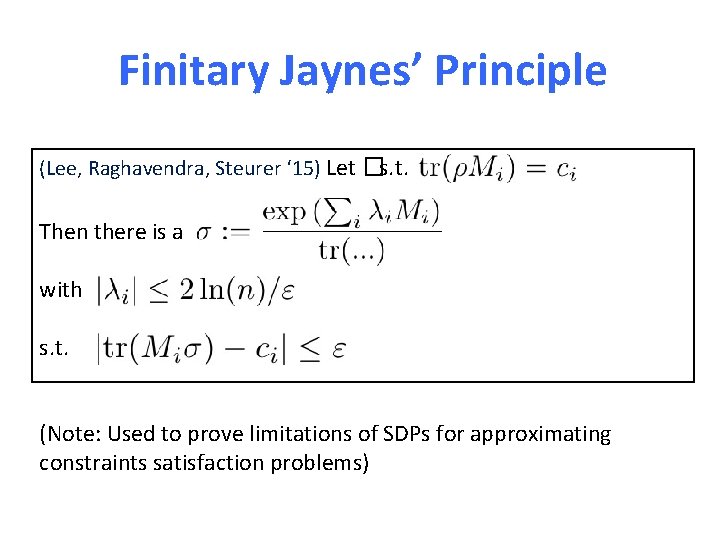
Finitary Jaynes’ Principle (Lee, Raghavendra, Steurer ‘ 15) Let �s. t. Then there is a with s. t. (Note: Used to prove limitations of SDPs for approximating constraints satisfaction problems)

Implementing Oracle by Gibbs Sampling Claim There is a Y of the form with x, y < log(n)/ε and N < α s. t. N < α:

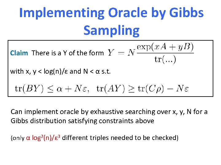
Implementing Oracle by Gibbs Sampling Claim There is a Y of the form with x, y < log(n)/ε and N < α s. t. Can implement oracle by exhaustive searching over x, y, N for a Gibbs distribution satisfying constraints above (only α log 2(n)/ε 3 different triples needed to be checked)

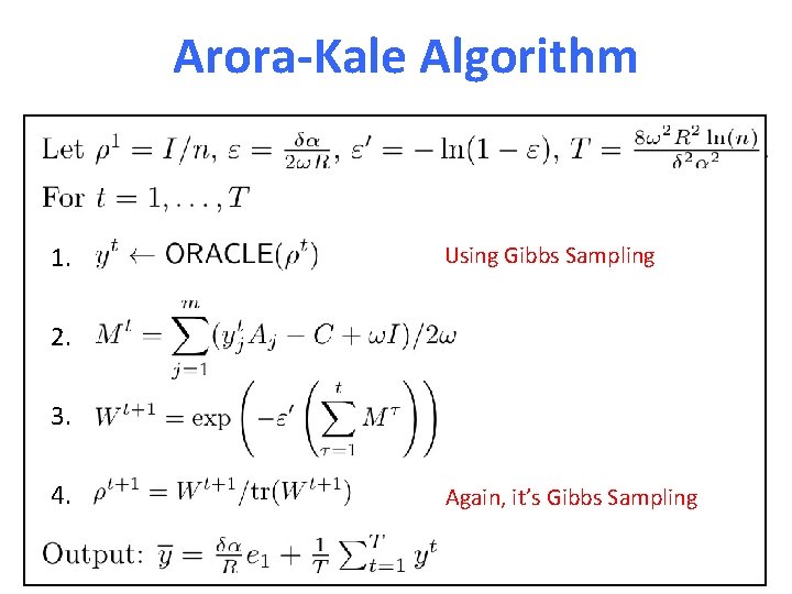
Arora-Kale Algorithm 1. Using Gibbs Sampling 2. 3. 4. Again, it’s Gibbs Sampling

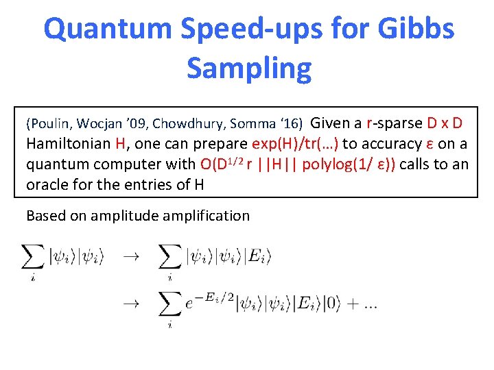
Quantum Speed-ups for Gibbs Sampling (Poulin, Wocjan ’ 09, Chowdhury, Somma ‘ 16) Given a r-sparse D x D Hamiltonian H, one can prepare exp(H)/tr(…) to accuracy ε on a quantum computer with O(D 1/2 r ||H|| polylog(1/ ε)) calls to an oracle for the entries of H Based on amplitude amplification

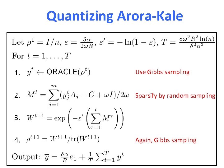
Quantizing Arora-Kale 1. Use Gibbs Sampling 2. 3. 4. Again, Gibbs Sampling

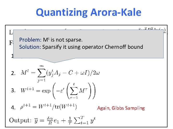
Quantizing Arora-Kale Problem: Mt is not sparse. Solution: Sparsify it using operator Chernoff bound 1. Using Gibbs Sampling 2. 3. 4. Again, Gibbs Sampling

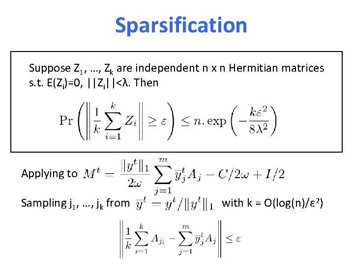
Sparsification Suppose Z 1, …, Zk are independent n x n Hermitian matrices s. t. E(Zi)=0, ||Zi||<λ. Then Applying to Sampling j 1, …, jk from with k = O(log(n)/ε 2)

Quantizing Arora-Kale 1. Use Gibbs sampling 2. Sparsify by random sampling 3. 4. Again, Gibbs sampling

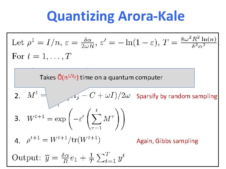
Quantizing Arora-Kale 1. 2. Takes Õ(n 1/2 r) Use Gibbs sampling time on a quantum computer Sparsify by random sampling 3. 4. Again, Gibbs sampling

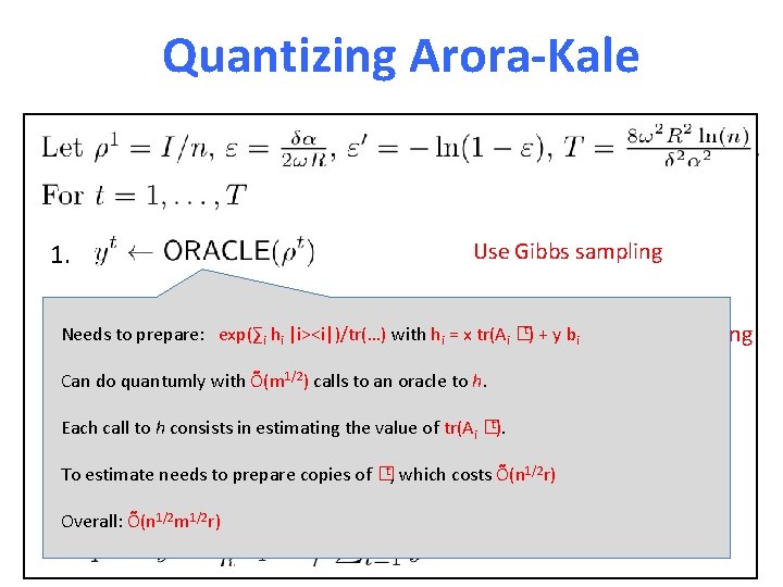
Quantizing Arora-Kale Use Gibbs sampling 1. 2. Needs to prepare: exp(∑i hi |i><i|)/tr(…) with hi = x Sparsify tr(Ai �t) + yby bi random sampling Can do quantumly with Õ(m 1/2) calls to an oracle to h. 3. Each call to h consists in estimating the value of tr(Ai �t). To estimate needs to prepare copies of �t, which costs Õ(n 1/2 r) 4. Overall: Õ(n 1/2 m 1/2 r)

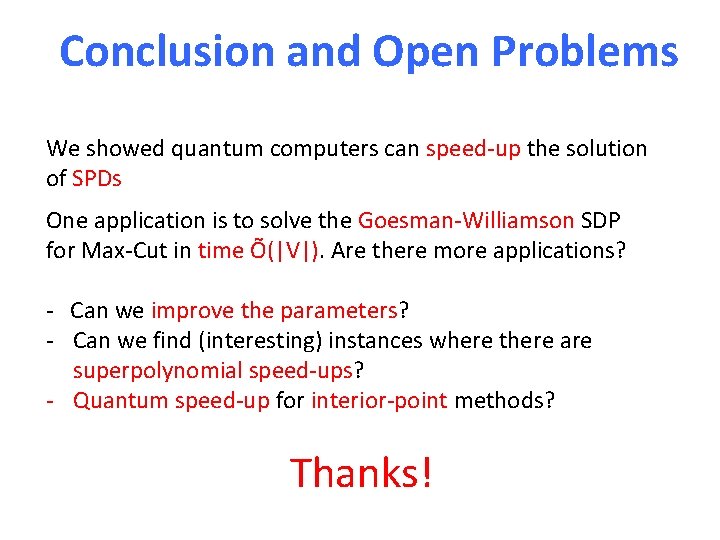
Conclusion and Open Problems We showed quantum computers can speed-up the solution of SPDs One application is to solve the Goesman-Williamson SDP for Max-Cut in time Õ(|V|). Are there more applications? - Can we improve the parameters? - Can we find (interesting) instances where there are superpolynomial speed-ups? - Quantum speed-up for interior-point methods? Thanks!