Graph Laplacian Regularization for LargeScale Semidefinite Programming Kilian

Graph Laplacian Regularization for Large-Scale Semidefinite Programming Kilian Weinberger et al. NIPS 2006 presented by Aggeliki Tsoli 3/21/2007

Introduction n Problem n n Current Approach n n n discovery of low dimensional representations of highdimensional data in many cases, local proximity measurements also available e. g. computer vision, sensor localization semidefinite programs (SDPs) – convex optimization Disadvantage: it doesn’t scale well for large inputs Paper Contribution n n 3/21/2007 method for solving very large problems of the above type much smaller/faster SDPs than those previously studied 2

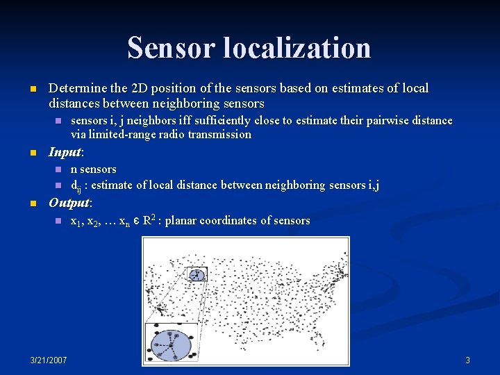
Sensor localization n Determine the 2 D position of the sensors based on estimates of local distances between neighboring sensors n n Input: n n n sensors i, j neighbors iff sufficiently close to estimate their pairwise distance via limited-range radio transmission n sensors dij : estimate of local distance between neighboring sensors i, j Output: n 3/21/2007 x 1, x 2, … xn є R 2 : planar coordinates of sensors 3

Work so far… n Minimize sum-of-squares loss function (1) n Centering constraint (assuming no sensor location is known in advance) (2) n Optimization in (1) non convex Likely to be trapped in local minima ! 3/21/2007 4

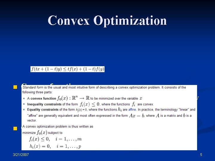
Convex Optimization n Convex function n a real-valued function f defined on a domain C that for any two points x and y in C and any t in [0, 1], n n Convex optimization 3/21/2007 5

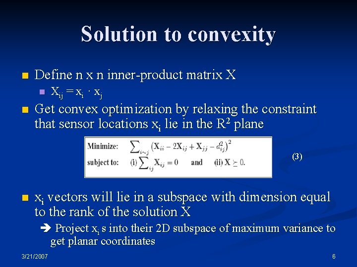
Solution to convexity n Define n x n inner-product matrix X n n Xij = xi · xj Get convex optimization by relaxing the constraint that sensor locations xi lie in the R 2 plane (3) n xi vectors will lie in a subspace with dimension equal to the rank of the solution X Project xi s into their 2 D subspace of maximum variance to get planar coordinates 3/21/2007 6

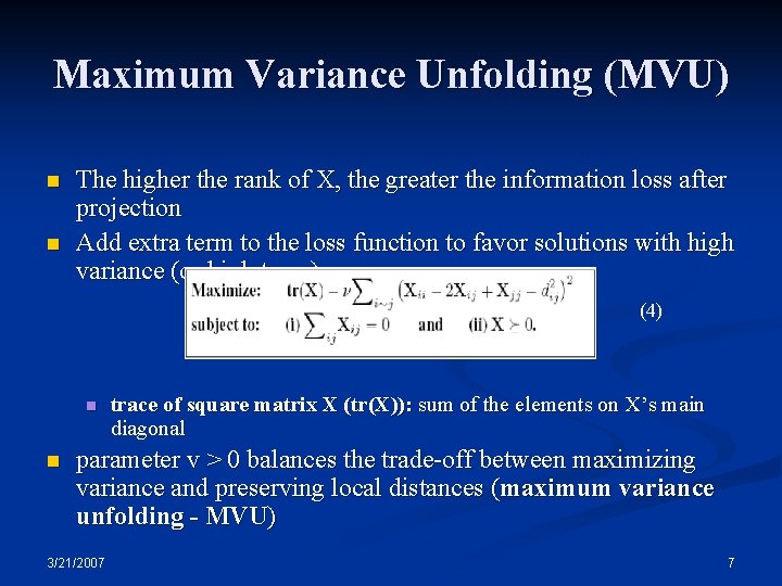
Maximum Variance Unfolding (MVU) n n The higher the rank of X, the greater the information loss after projection Add extra term to the loss function to favor solutions with high variance (or high trace) (4) n n trace of square matrix X (tr(X)): sum of the elements on X’s main diagonal parameter v > 0 balances the trade-off between maximizing variance and preserving local distances (maximum variance unfolding - MVU) 3/21/2007 7

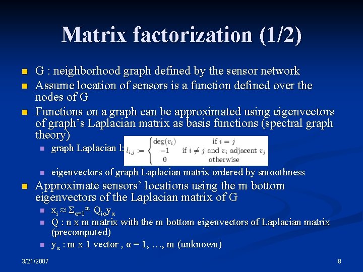
Matrix factorization (1/2) n n G : neighborhood graph defined by the sensor network Assume location of sensors is a function defined over the nodes of G Functions on a graph can be approximated using eigenvectors of graph’s Laplacian matrix as basis functions (spectral graph theory) n graph Laplacian l: n eigenvectors of graph Laplacian matrix ordered by smoothness Approximate sensors’ locations using the m bottom eigenvectors of the Laplacian matrix of G n n n 3/21/2007 xi ≈ Σα=1 m Qiαyα Q : n x m matrix with the m bottom eigenvectors of Laplacian matrix (precomputed) yα : m x 1 vector , α = 1, …, m (unknown) 8

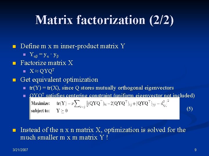
Matrix factorization (2/2) n Define m x m inner-product matrix Y n n Factorize matrix X n n Yαβ = yα · yβ X ≈ QYQT Get equivalent optimization n n tr(Y) = tr(X), since Q stores mutually orthogonal eigenvectors QYQT satisfies centering constraint (uniform eigenvector not included) (5) n Instead of the n x n matrix X, optimization is solved for the much smaller m x m matrix Y ! 3/21/2007 9

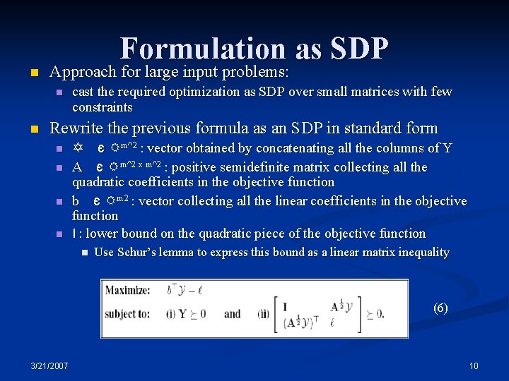
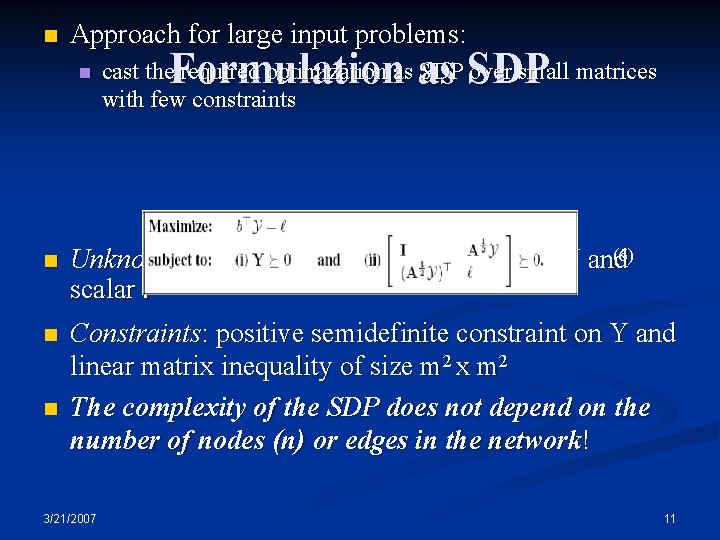
n Formulation as SDP Approach for large input problems: n n cast the required optimization as SDP over small matrices with few constraints Rewrite the previous formula as an SDP in standard form n n Y є Rm^2 : vector obtained by concatenating all the columns of Y A є Rm^2 x m^2 : positive semidefinite matrix collecting all the quadratic coefficients in the objective function b є Rm 2 : vector collecting all the linear coefficients in the objective function l : lower bound on the quadratic piece of the objective function n Use Schur’s lemma to express this bound as a linear matrix inequality (6) 3/21/2007 10

n Approach for large input problems: n Formulation as SDP cast the required optimization as SDP over small matrices with few constraints n (6) Unknown variables: m(m+1)/2 elements of Y and scalar l n Constraints: positive semidefinite constraint on Y and linear matrix inequality of size m 2 x m 2 The complexity of the SDP does not depend on the number of nodes (n) or edges in the network! n 3/21/2007 11

Gradient-based improvement n 2 -step process (optional): Starting from the m-dimensional solution of eq. (6), use conjugate gradient methods to maximize the objective function in eq. (4) n Project the results from the previous step into the R 2 plane and use conjugate gradient methods to minimize the loss function in eq. (1) n n conjugate gradient method: iterative method for minimizing a quadratic function where its Hessian matrix (matrix of second partial derivatives) is positive definite 3/21/2007 12

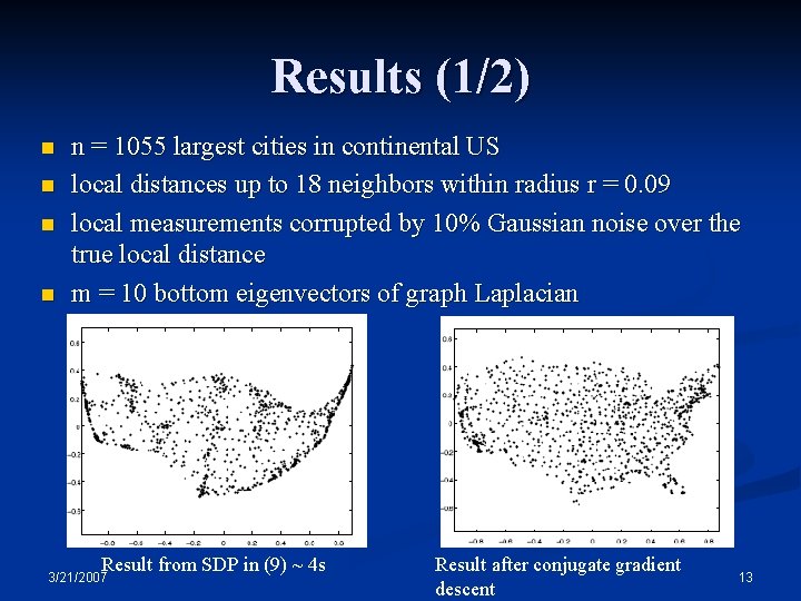
Results (1/2) n n n = 1055 largest cities in continental US local distances up to 18 neighbors within radius r = 0. 09 local measurements corrupted by 10% Gaussian noise over the true local distance m = 10 bottom eigenvectors of graph Laplacian Result from SDP in (9) ~ 4 s 3/21/2007 Result after conjugate gradient descent 13

Results (2/2) n n n = 20, 000 uniformly sampled points inside the unit square local distances up to 20 other nodes within radius r = 0. 06 m = 10 bottom eigenvectors of graph Laplacian 19 s to construct and solve the SDP 52 s for 100 iterations in conjugate gradient descent 3/21/2007 14

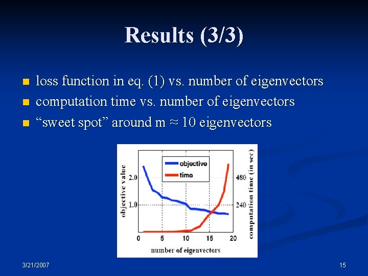
Results (3/3) n n n loss function in eq. (1) vs. number of eigenvectors computation time vs. number of eigenvectors “sweet spot” around m ≈ 10 eigenvectors 3/21/2007 15

Fast. MVU on Robotics n Control of a robot using sparse user input n n e. g. 2 D mouse position Robot localization n 3/21/2007 the robot’s location is inferred from the high dimensional description of its state in terms of sensorimotor input 16

Conclusion Approach for inferring low dimensional representations from local distance constraints using MVU n Use of matrix factorization computed from the bottom eigenvectors of the graph Laplacian n Local search methods can refine solution n Suitable for large input; its complexity does not depend on the input! n 3/21/2007 17