Elements of Graph Theory l A graph G

Elements of Graph Theory l. A graph G = (V, E) consists of a vertex set V and an edge set E. l If G is a directed graph, each edge is an ordered pair of vertices l A bipartite graph is one in which the vertices can be divided into two groups, so that all edges join vertices in different groups.

העברת הנק' לגרף קבע את הנק' במישור קבע מרחק בין כל זוג נקודות 0 1 1. 5 2 5 6 7 9 1 0 2 1 6. 5 6 8 8 1. 5 2 0 1 4 4 6 5. 5. . . n-D data points graph representation distance matrix l l

Minimal Cut l l Create a graph G(V, E) from the data Compute all the distances in the graph The weight of each edge is the distance Remove edges from the graph according to some threshold

Similarity Graph l l Distance decrease similarty increase Represent dataset as a weighted graph G(V, E) V={xi} Set of n vertices representing data points E={Wij} Set of weighted edges indicating pair-wise similarity between points 0. 1 0. 8 5 1 0. 8 0. 6 2 6 4 0. 8 3 0. 2 0. 7

Similarity Graph l l l Wij represent similarity between vertex If Wij=0 where isn’t similarity Wii=0

Graph Partitioning l Clustering can be viewed as partitioning a similarity graph l Bi-partitioning task: l Divide vertices into two disjoint groups (A, B) A 1 2 4 3 V=A U B B 5 6

Clustering Objectives l Traditional definition of a “good” clustering: 1. 2. l Points assigned to same cluster should be highly similar. Points assigned to different clusters should be highly dissimilar. Apply these objectives to our graph representation 0. 8 0. 1 1 5 0. 8 0. 6 2 0. 8 3 6 4 0. 7 0. 2 Minimize weight of between-group connections

Graph Cuts l l Express partitioning objectives as a function of the “edge cut” of the partition. Cut: Set of edges with only one vertex in a group. we wants to find the minimal cut beetween groups. The groups that has the minimal cut would be the partition A B 0. 1 0. 8 1 0. 6 2 0. 8 3 5 0. 8 6 4 0. 2 0. 8 0. 7 cut(A, B) = 0. 3

Graph Cut Criteria l Criterion: Minimum-cut l Minimise weight of connections between groups min cut(A, B) l l Degenerate case: Optimal cut Minimum cut Problem: l l Only considers external cluster connections Does not consider internal cluster density

Graph Cut Criteria (continued) l Criterion: Normalised-cut (Shi & Malik, ’ 97) l Consider the connectivity between groups relative to the density of each group. l Normalise the association between groups by volume. l Vol(A): The total weight of the edges originating from group A. l Why use this criterion? l l Minimising the normalised cut is equivalent to maximising normalised association. Produces more balanced partitions.

Example b 4 2 i 11 a h 1 4 b h 8 g c 2 1 e 7 4 f d 9 14 6 7 8 9 10 2 i 11 d 14 4 8 4 7 6 7 8 a c 8 10 g 2 f e

Example 4 8 b 4 c 2 i 11 a 8 h 8 1 g 8 h 8 2 f 7 7 4 d 1 g 9 14 6 7 8 c 2 2 i 11 a e 10 8 4 9 14 4 4 b d 6 7 8 7 10 2 f 4 e

Example 4 8 b 4 2 i 11 a h 87 c g 6 8 7 1 e 14 2 f 4 7 7 d 9 10 g 6 2 2 f 4 10 e 14 4 6 7 h c 2 2 i 11 9 10 8 4 d 4 1 b 8 7 2 4 a 7 6 7 8 8

Example 8 4 8 b 4 h 7 1 4 8 4 h 1 2 1 e f 2 4 8 7 c 7 d 9 10 g 2 2 f 4 10 e 14 4 6 7 8 10 10 2 2 i 11 a 9 14 4 g 1 b d 6 7 8 7 c 2 2 i 11 a 7

Example 8 4 8 b 4 2 2 i 11 a h 1 7 d 1 9 9 10 e 14 4 6 7 8 c 7 10 g 2 2 f 4

Similarity Graph l l l Wij represent similarity between vertex If Wij=0 where isn’t similarity Wii=0

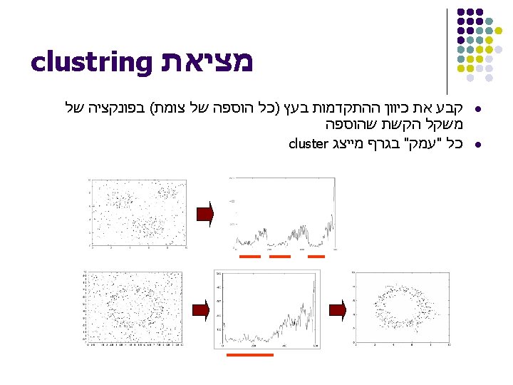
Example – 2 Spirals Dataset exhibits complex cluster shapes Þ K-means performs very poorly in this space due bias toward dense spherical clusters. In the embedded space given by two leading eigenvectors, clusters are trivial to separate.

Spectral Graph Theory l Possible approach l l Represent a similarity graph as a matrix Apply knowledge from Linear Algebra… l The eigenvalues and eigenvectors of a matrix provide global information about its structure. l Spectral Graph Theory l l Analyse the “spectrum” of matrix representing a graph. Spectrum : The eigenvectors of a graph, ordered by the magnitude(strength) of their corresponding eigenvalues.

Matrix Representations Adjacency matrix (A) l n x n matrix l : edge weight between vertex xi and xj l 0. 1 0. 8 5 1 0. 8 0. 6 2 0. 8 l 0. 8 6 4 0. 7 3 0. 2 Important properties: l Þ Þ x 1 x 2 x 3 x 4 x 5 x 6 x 1 0 0. 8 0. 6 0 0. 1 0 x 2 0. 8 0 0 0 x 3 0. 6 0. 8 0 0. 2 0 0 x 4 0 0 0. 2 0 0. 8 0. 7 x 5 0. 1 0 0 0. 8 x 6 0 0. 7 0. 8 0 Symmetric matrix Eigenvalues are real Eigenvector could span orthogonal base

Matrix Representations (continued) l Degree matrix (D) l n x n diagonal matrix : total weight of edges incident to vertex xi l 0. 1 5 1 0. 8 0. 6 2 0. 8 l 3 0. 8 6 4 0. 2 0. 7 Important application: l Normalise adjacency matrix x 1 x 2 x 3 x 4 x 5 x 6 x 1 1. 5 0 0 0 x 2 0 1. 6 0 0 x 3 0 0 1. 6 0 0 0 x 4 0 0 0 1. 7 0 0 x 5 0 0 1. 7 0 x 6 0 0 0 1. 5

Matrix Representations (continued) l Laplacian matrix (L) l n x n symmetric matrix 0. 1 5 1 0. 8 0. 6 2 0. 8 3 4 0. 2 Important properties: l l l x 1 x 2 x 3 x 4 x 5 x 6 x 1 1. 5 -0. 8 -0. 6 0 -0. 1 0 x 2 -0. 8 1. 6 -0. 8 0 0 0 x 3 -0. 6 -0. 8 1. 6 -0. 2 0 0 6 0. 7 0. 8 l L=D-A x 4 0 0 -0. 2 1. 7 -0. 8 -0. 7 x 5 -0. 1 0 0 0. 8 - 1. 7 -0. 8 x 6 0 0 0 -0. 7 -0. 8 1. 5 Eigenvalues are non-negative real numbers Eigenvectors are real and orthogonal Eigenvalues and eigenvectors provide an insight into the connectivity of the graph…

Another option – normalized laplasian l Laplacian matrix (L) l n x n symmetric matrix 0. 1 5 1 0. 8 0. 6 2 6 4 0. 7 0. 8 l 0. 8 3 0. 2 Important properties: l l 1. 00 -0. 52 -0. 39 0. 00 -0. 06 0. 00 -0. 52 1. 00 -0. 50 0. 00 -0. 39 -0. 50 1. 00 0. 00 -0. 12 1. 00 -0. 47 -0. 44 -0. 06 0. 00 0. 47 - 1. 00 -0. 50 0. 00 -0. 44 -0. 50 1. 00 Eigenvectors are real and normalize Each Aij which i, j is not equal = -0. 12

Spectral Clustering Algorithms l Three basic stages: 1. Pre-processing l 2. Decomposition l l 3. Construct a matrix representation of the dataset. Compute eigenvalues and eigenvectors of the matrix. Map each point to a lower-dimensional representation based on one or more eigenvectors. Grouping l Assign points to two or more clusters, based on the new representation.

Spectral Bi-partitioning Algorithm x 1 Pre-processing 1. l Build Laplacian matrix L of the graph Decomposition 2. l l Find eigenvalues X and eigenvectors Λ of the matrix L Map vertices to corresponding components of λ 2 Λ= x 2 x 3 x 4 x 5 x 6 x 1 1. 5 -0. 8 -0. 6 0 -0. 1 0 x 2 -0. 8 1. 6 -0. 8 0 0 0 x 3 -0. 6 -0. 8 1. 6 -0. 2 0 0 x 4 0 0 -0. 2 1. 7 -0. 8 -0. 7 x 5 -0. 1 0 0 -0. 8 1. 7 -0. 8 x 6 0 0 0 -0. 7 -0. 8 1. 5 0. 0 0. 4 0. 2 0. 1 0. 4 -0. 2 -0. 9 0. 4 0. 2 0. 1 -0. 0. 4 0. 3 0. 4 0. 2 -0. 2 0. 0 -0. 2 0. 6 0. 4 -0. 4 0. 9 0. 2 -0. 4 -0. 6 2. 5 0. 4 -0. 7 -0. 4 -0. 8 -0. 6 -0. 2 3. 0 0. 4 -0. 7 -0. 2 0. 5 0. 8 0. 9 2. 2 2. 3 x 1 0. 2 x 2 0. 2 x 3 0. 2 x 4 -0. 4 x 5 -0. 7 x 6 -0. 7 X=

Spectral Bi-partitioning Algorithm The matrix which represents the eigenvector of the laplacian the eigenvector matched to the corresponded eigenvalues with increasing order 0. 41 -0. 65 -0. 31 -0. 38 0. 11 0. 41 -0. 44 0. 01 0. 30 0. 71 0. 22 0. 41 -0. 37 0. 64 0. 04 -0. 39 -0. 37 0. 41 0. 37 0. 34 -0. 45 0. 00 0. 61 0. 41 -0. 17 -0. 30 0. 35 -0. 65 0. 41 0. 45 -0. 18 0. 72 -0. 29 0. 09

Spectral Bi-partitioning (continued) Grouping l l l Sort components of reduced 1 -dimensional vector. Identify clusters by splitting the sorted vector in two. How to choose a splitting point? l l Naïve approaches: l l Split at 0, mean or median value More expensive approaches l Attempt to minimise normalised cut criterion in 1 -dimension x 1 0. 2 Split at 0 x 2 0. 2 x 3 0. 2 Cluster A: Positive points Cluster B: Negative points x 4 -0. 4 x 5 -0. 7 x 1 0. 2 x 4 -0. 4 x 6 -0. 7 x 2 0. 2 x 5 -0. 7 x 3 0. 2 x 6 -0. 7 A B