Today Local invariant features Detection of interest points

Today • Local invariant features – Detection of interest points • Harris corner detection – Scale Estimation

• What would we like our local features to be invariant to? • • • Geometric Photometric Noise Blur Compression Artifacts

Main questions • Where will the interest points come from? – What are salient features that we’ll detect in multiple views? • How to describe a local region? • How to establish correspondences, i. e. , compute matches?

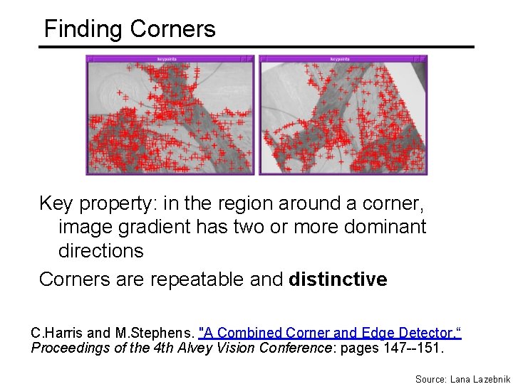
Finding Corners Key property: in the region around a corner, image gradient has two or more dominant directions Corners are repeatable and distinctive C. Harris and M. Stephens. "A Combined Corner and Edge Detector. “ Proceedings of the 4 th Alvey Vision Conference: pages 147 --151. Source: Lana Lazebnik

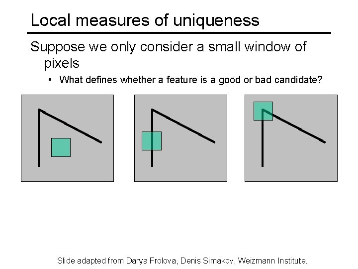
Local measures of uniqueness Suppose we only consider a small window of pixels • What defines whether a feature is a good or bad candidate? Slide adapted from Darya Frolova, Denis Simakov, Weizmann Institute.

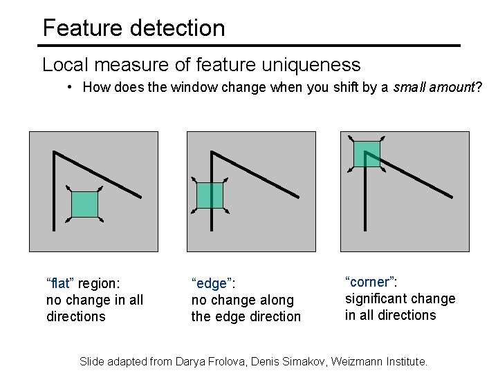
Feature detection Local measure of feature uniqueness • How does the window change when you shift by a small amount? “flat” region: no change in all directions “edge”: no change along the edge direction “corner”: significant change in all directions Slide adapted from Darya Frolova, Denis Simakov, Weizmann Institute.

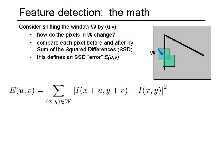
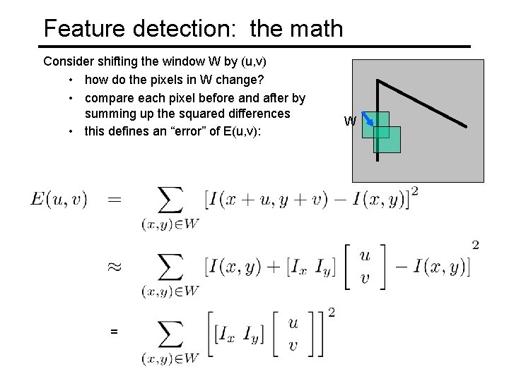
Feature detection: the math Consider shifting the window W by (u, v) • how do the pixels in W change? • compare each pixel before and after by Sum of the Squared Differences (SSD) • this defines an SSD “error” E(u, v): W

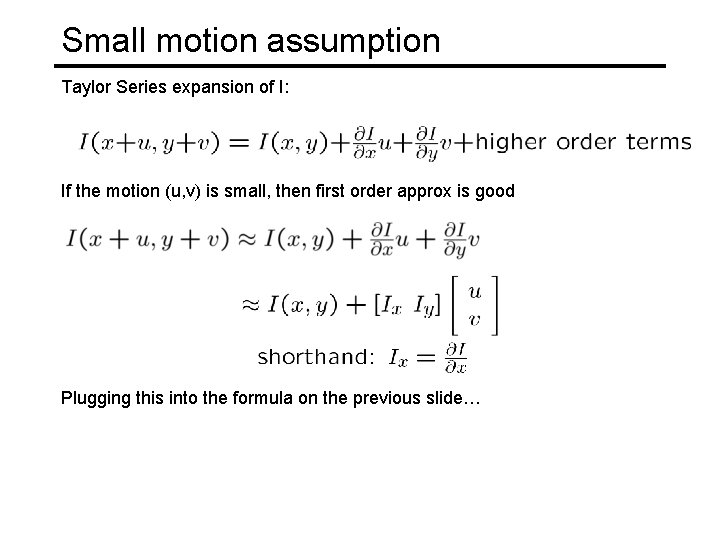
Small motion assumption Taylor Series expansion of I: If the motion (u, v) is small, then first order approx is good Plugging this into the formula on the previous slide…

Feature detection: the math Consider shifting the window W by (u, v) • how do the pixels in W change? • compare each pixel before and after by summing up the squared differences • this defines an “error” of E(u, v): = W

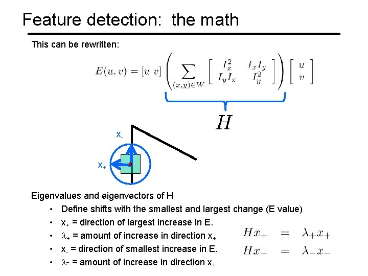
Quick eigenvalue/eigenvector review The eigenvectors of a matrix A are the vectors x that satisfy: The scalar is the eigenvalue corresponding to x • The eigenvalues are found by solving: • In our case, A = H is a 2 x 2 matrix, so we have • The solution: Once you know , you find x by solving

Feature detection: the math This can be rewritten: x x+ Eigenvalues and eigenvectors of H • Define shifts with the smallest and largest change (E value) • x+ = direction of largest increase in E. • + = amount of increase in direction x+ • x- = direction of smallest increase in E. • - = amount of increase in direction x+

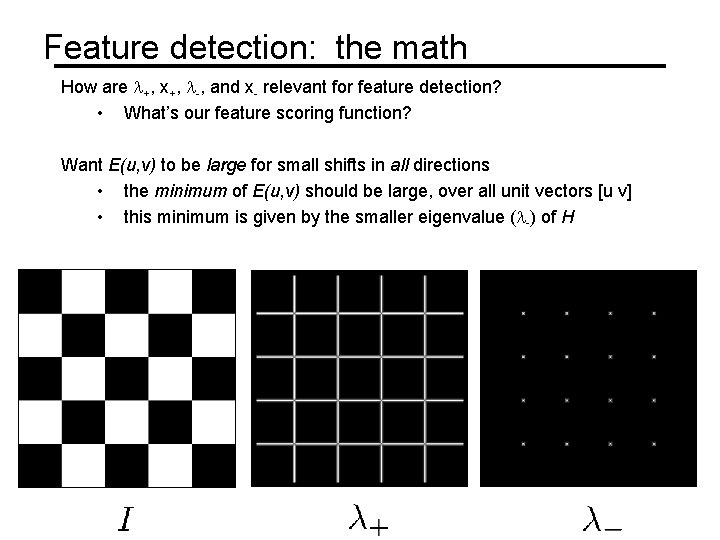
Feature detection: the math How are +, x+, -, and x- relevant for feature detection? • What’s our feature scoring function? Want E(u, v) to be large for small shifts in all directions • the minimum of E(u, v) should be large, over all unit vectors [u v] • this minimum is given by the smaller eigenvalue ( -) of H

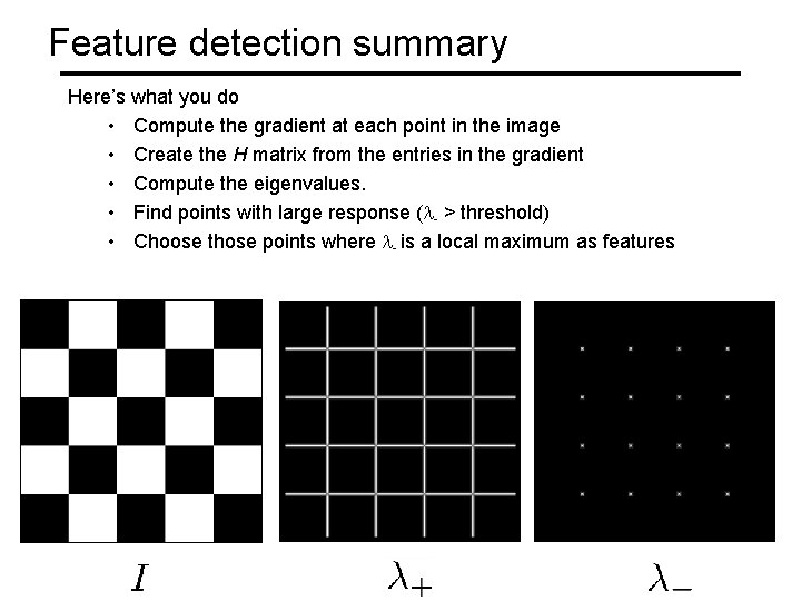
Feature detection summary Here’s what you do • Compute the gradient at each point in the image • Create the H matrix from the entries in the gradient • Compute the eigenvalues. • Find points with large response ( - > threshold) • Choose those points where - is a local maximum as features

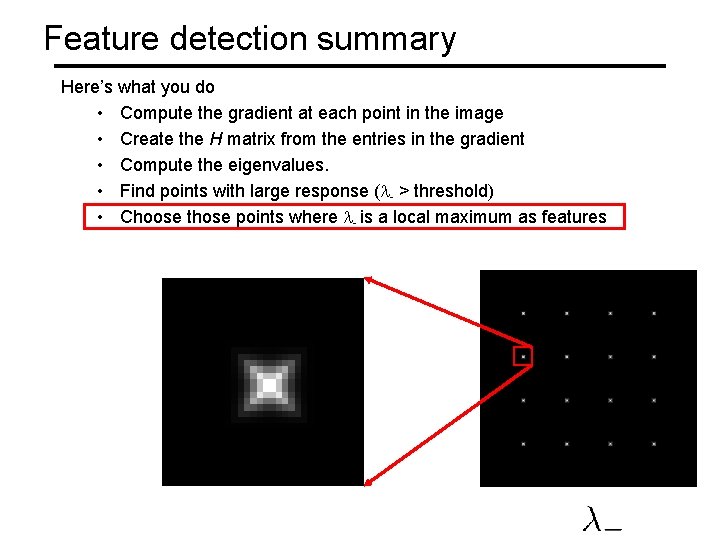
Feature detection summary Here’s what you do • Compute the gradient at each point in the image • Create the H matrix from the entries in the gradient • Compute the eigenvalues. • Find points with large response ( - > threshold) • Choose those points where - is a local maximum as features

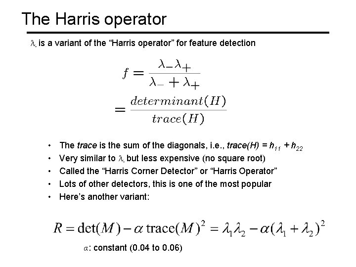
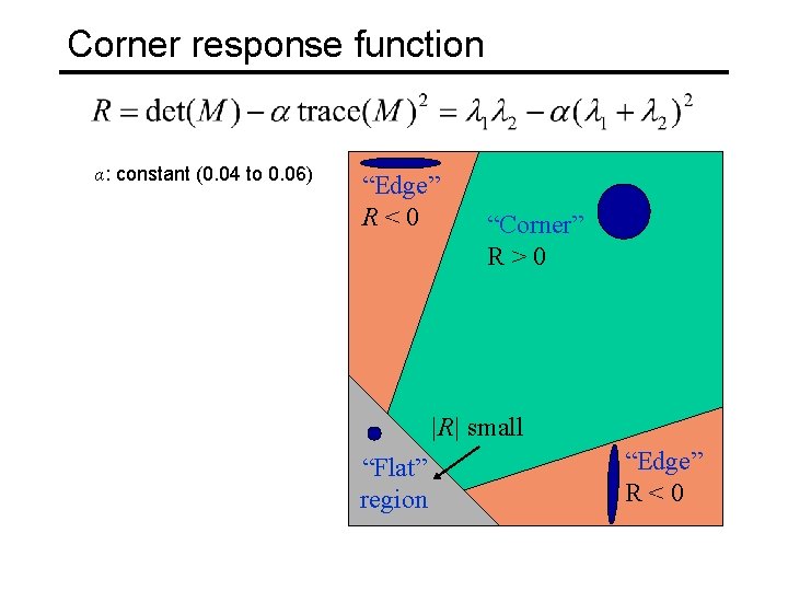
The Harris operator - is a variant of the “Harris operator” for feature detection • • • The trace is the sum of the diagonals, i. e. , trace(H) = h 11 + h 22 Very similar to - but less expensive (no square root) Called the “Harris Corner Detector” or “Harris Operator” Lots of other detectors, this is one of the most popular Here’s another variant: α: constant (0. 04 to 0. 06)

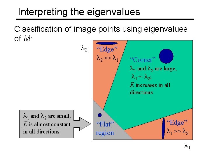
Interpreting the eigenvalues Classification of image points using eigenvalues of M: 2 “Edge” 2 >> 1 “Corner” 1 and 2 are large, 1 ~ 2; E increases in all directions 1 and 2 are small; E is almost constant in all directions “Flat” region “Edge” 1 >> 2 1

Corner response function α: constant (0. 04 to 0. 06) “Edge” R<0 “Corner” R>0 |R| small “Flat” region “Edge” R<0

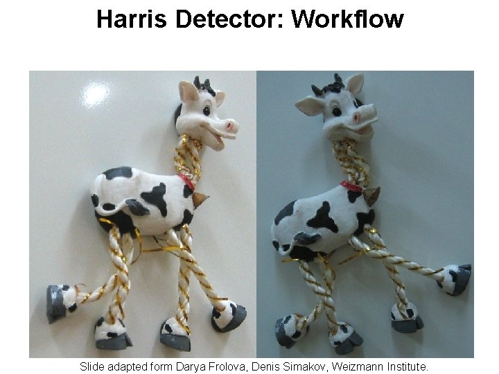
Harris Detector: Workflow Slide adapted form Darya Frolova, Denis Simakov, Weizmann Institute.

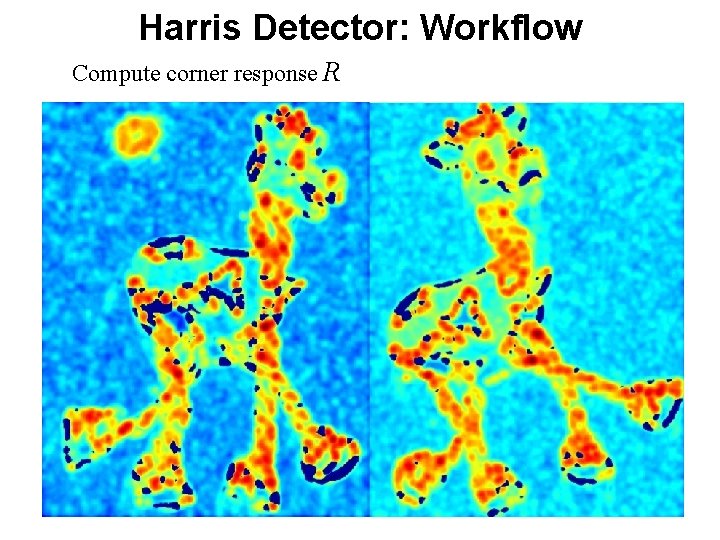
Harris Detector: Workflow Compute corner response R

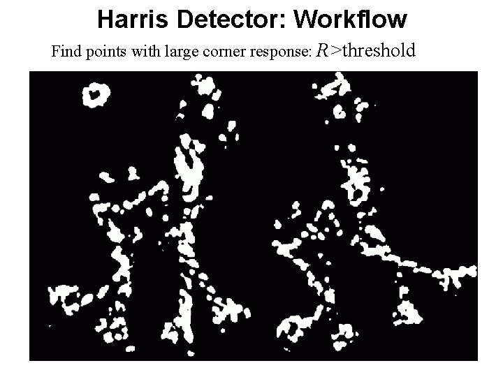
Harris Detector: Workflow Find points with large corner response: R>threshold

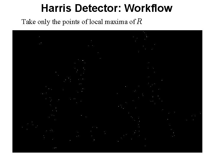
Harris Detector: Workflow Take only the points of local maxima of R

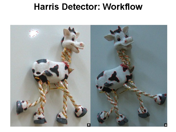
Harris Detector: Workflow

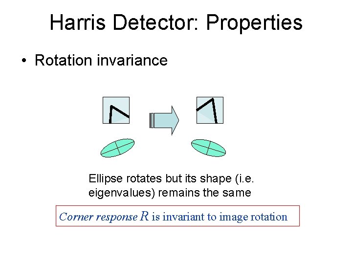
Harris Detector: Properties • Rotation invariance Ellipse rotates but its shape (i. e. eigenvalues) remains the same Corner response R is invariant to image rotation

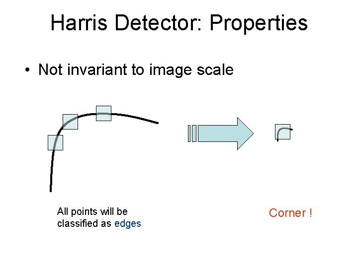
Harris Detector: Properties • Not invariant to image scale All points will be classified as edges Corner !

• How can we detect scale invariant interest points?

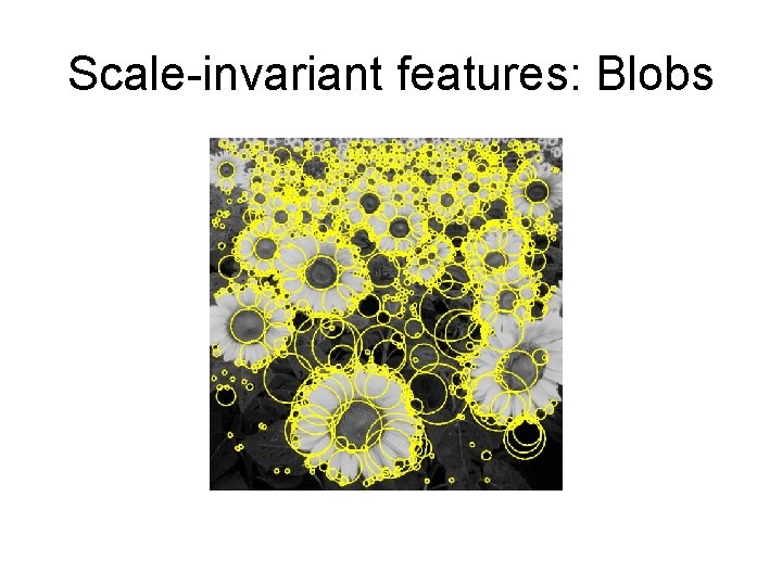
Scale-invariant features: Blobs

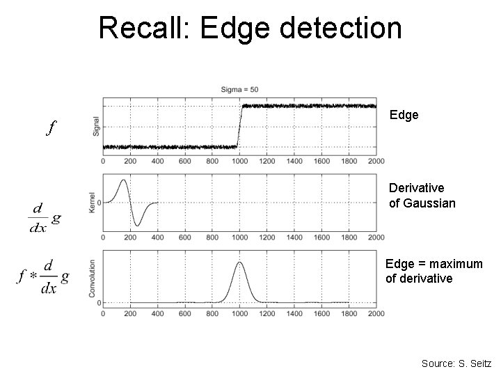
Recall: Edge detection f Edge Derivative of Gaussian Edge = maximum of derivative Source: S. Seitz

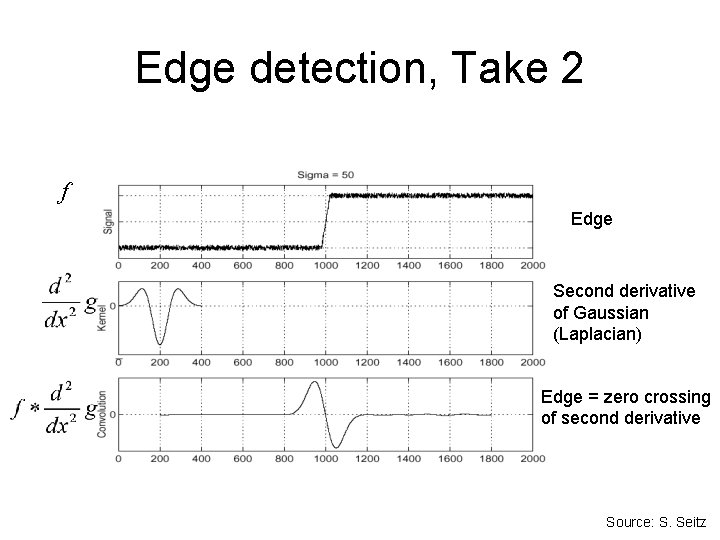
Edge detection, Take 2 f Edge Second derivative of Gaussian (Laplacian) Edge = zero crossing of second derivative Source: S. Seitz

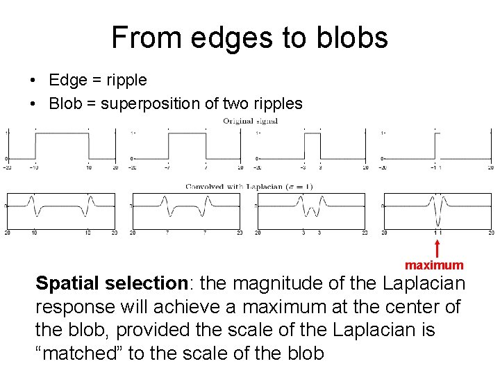
From edges to blobs • Edge = ripple • Blob = superposition of two ripples maximum Spatial selection: the magnitude of the Laplacian response will achieve a maximum at the center of the blob, provided the scale of the Laplacian is “matched” to the scale of the blob

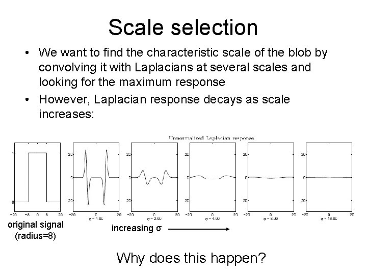
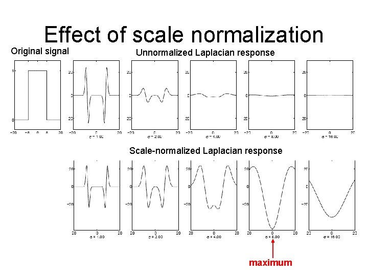
Scale selection • We want to find the characteristic scale of the blob by convolving it with Laplacians at several scales and looking for the maximum response • However, Laplacian response decays as scale increases: original signal (radius=8) increasing σ Why does this happen?

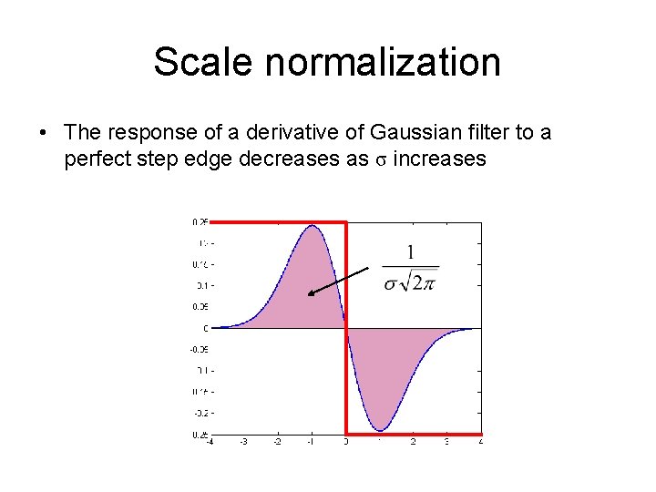
Scale normalization • The response of a derivative of Gaussian filter to a perfect step edge decreases as σ increases

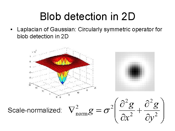
Scale normalization • The response of a derivative of Gaussian filter to a perfect step edge decreases as σ increases • To keep response the same (scale-invariant), must multiply Gaussian derivative by σ • Laplacian is the second Gaussian derivative, so it must be multiplied by σ2

Effect of scale normalization Original signal Unnormalized Laplacian response Scale-normalized Laplacian response maximum

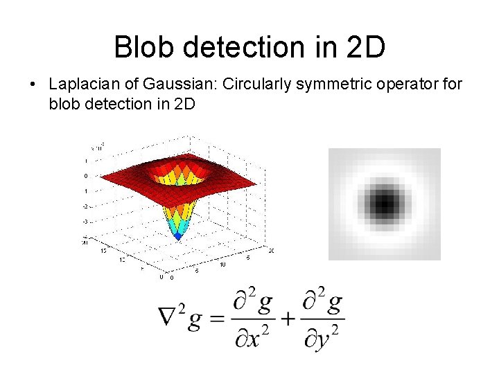
Blob detection in 2 D • Laplacian of Gaussian: Circularly symmetric operator for blob detection in 2 D

Blob detection in 2 D • Laplacian of Gaussian: Circularly symmetric operator for blob detection in 2 D Scale-normalized:

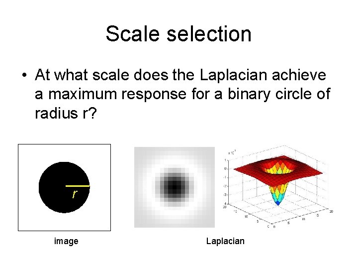
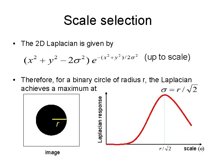
Scale selection • At what scale does the Laplacian achieve a maximum response for a binary circle of radius r? r image Laplacian

Scale selection • The 2 D Laplacian is given by (up to scale) r image Laplacian response • Therefore, for a binary circle of radius r, the Laplacian achieves a maximum at scale (σ)

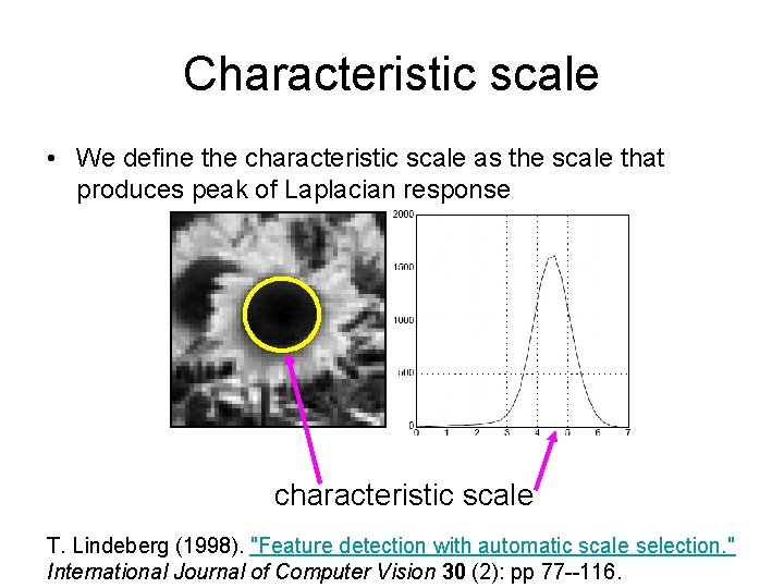
Characteristic scale • We define the characteristic scale as the scale that produces peak of Laplacian response characteristic scale T. Lindeberg (1998). "Feature detection with automatic scale selection. " International Journal of Computer Vision 30 (2): pp 77 --116.

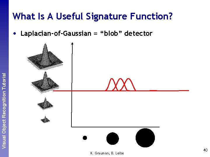
What Is A Useful Signature Function? Perceptual and. Recognition Sensory Augmented Visual Object Tutorial Computing • Laplacian-of-Gaussian = “blob” detector K. Grauman, B. Leibe 40

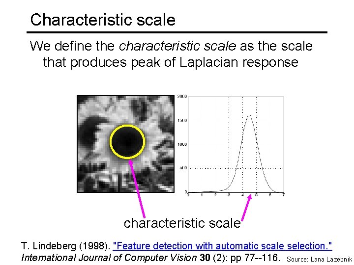
Characteristic scale We define the characteristic scale as the scale that produces peak of Laplacian response characteristic scale T. Lindeberg (1998). "Feature detection with automatic scale selection. " International Journal of Computer Vision 30 (2): pp 77 --116. Source: Lana Lazebnik

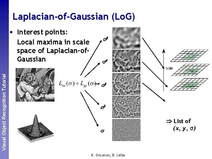
Laplacian-of-Gaussian (Lo. G) Perceptual and. Recognition Sensory Augmented Visual Object Tutorial Computing • Interest points: Local maxima in scale space of Laplacian-of. Gaussian s 5 s 4 s 3 s 2 s K. Grauman, B. Leibe List of (x, y, σ)

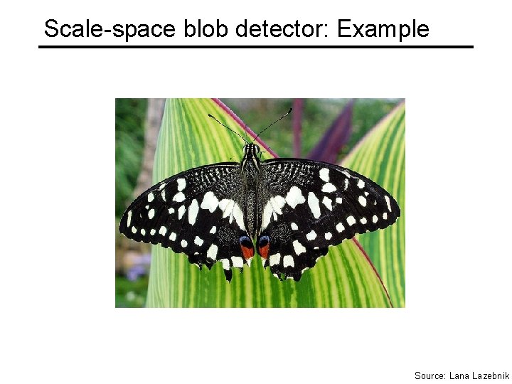
Scale-space blob detector: Example Source: Lana Lazebnik

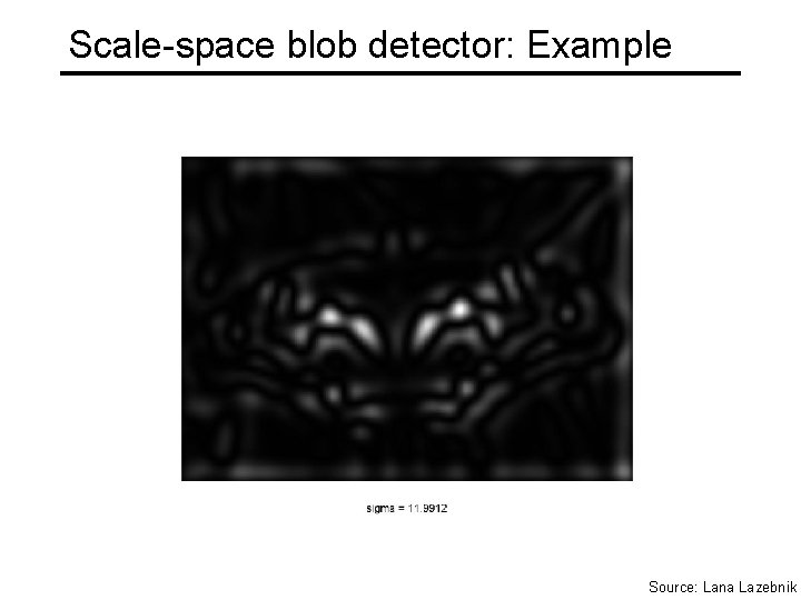
Scale-space blob detector: Example Source: Lana Lazebnik

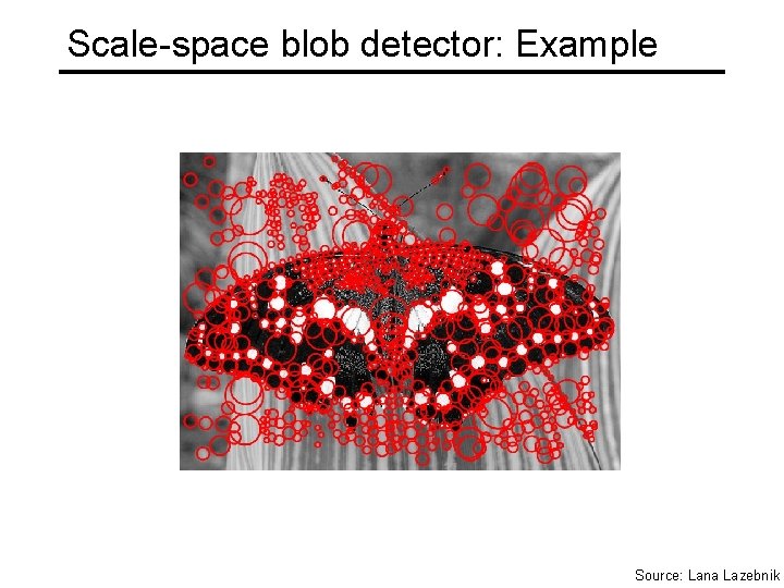
Scale-space blob detector: Example Source: Lana Lazebnik