PREDICT 422 Practical Machine Learning Module 4 Linear

PREDICT 422: Practical Machine Learning Module 4: Linear Model Selection and Regularization Lecturer: Nathan Bastian, Section: XXX

Assignment § Reading: Ch. 6 § Activity: Quiz 4, R Lab 4

References § An Introduction to Statistical Learning, with Applications in R (2013), by G. James, D. Witten, T. Hastie, and R. Tibshirani. § The Elements of Statistical Learning (2009), by T. Hastie, R. Tibshirani, and J. Friedman. § Learning from Data: A Short Course (2012), by Y. Abu-Mostafa, M. Magdon. Ismail, and H. Lin. § Machine Learning: A Probabilistic Perspective (2012), by K. Murphy.

Lesson Goals: § § § Understand best subset selection and stepwise selection methods for reducing the number of predictor variables in regression. Indirectly estimate test error by adjusting training error to account for bias due to overfitting (Cp, AIC, BIC, adjusted R 2). Directly estimate test error using validation set approach and crossvalidation approach. Understand know how to perform ridge regression and the lasso as shrinkage (regularization) methods. Understand know how to perform principal components regression and partial least squares as dimension reduction methods. Learn considerations for high-dimensional settings.

Improving the Linear Model § We may want to improve the simple linear model by replacing OLS estimation with some alternative fitting procedure. § Why use an alternative fitting procedure? – Prediction Accuracy – Model Interpretability

Prediction Accuracy § The OLS estimates have relatively low bias and low variability especially when the relationship between the response and predictors is linear and n >> p. § If n is not much larger than p, then the OLS fit can have high variance and may result in over fitting and poor estimates on unseen observations. § If p > n, then the variability of the OLS fit increases dramatically, and the variance of these estimates in infinite.

Model Interpretability § When we have a large number of predictors in the model, there will generally be many that have little or no effect on the response. § Including such irrelevant variable leads to unnecessary complexity. § Leaving these variables in the model makes it harder to see the effect of the important variables. § The model would be easier to interpret by removing (i. e. setting the coefficients to zero) the unimportant variables.

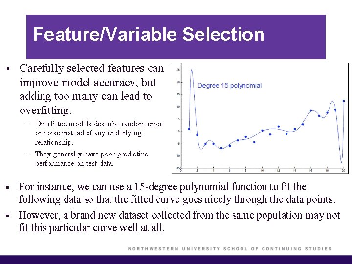
Feature/Variable Selection § Carefully selected features can improve model accuracy, but adding too many can lead to overfitting. – Overfitted models describe random error or noise instead of any underlying relationship. – They generally have poor predictive performance on test data. § § For instance, we can use a 15 -degree polynomial function to fit the following data so that the fitted curve goes nicely through the data points. However, a brand new dataset collected from the same population may not fit this particular curve well at all.

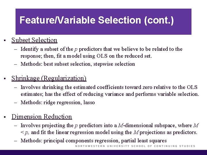
Feature/Variable Selection (cont. ) § Subset Selection – Identify a subset of the p predictors that we believe to be related to the response; then, fit a model using OLS on the reduced set. – Methods: best subset selection, stepwise selection § Shrinkage (Regularization) – Involves shrinking the estimated coefficients toward zero relative to the OLS estimates; has the effect of reducing variance and performs variable selection. – Methods: ridge regression, lasso § Dimension Reduction – Involves projecting the p predictors into a M-dimensional subspace, where M < p, and fit the linear regression model using the M projections as predictors. – Methods: principal components regression, partial least squares

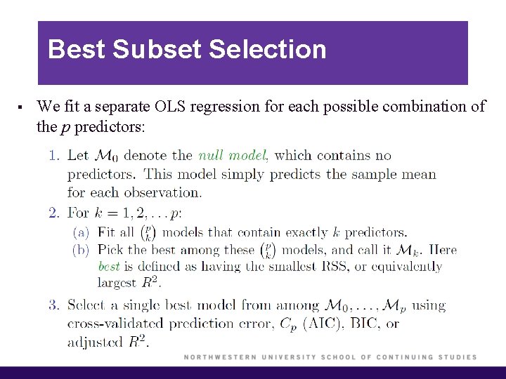
Best Subset Selection § We fit a separate OLS regression for each possible combination of the p predictors:

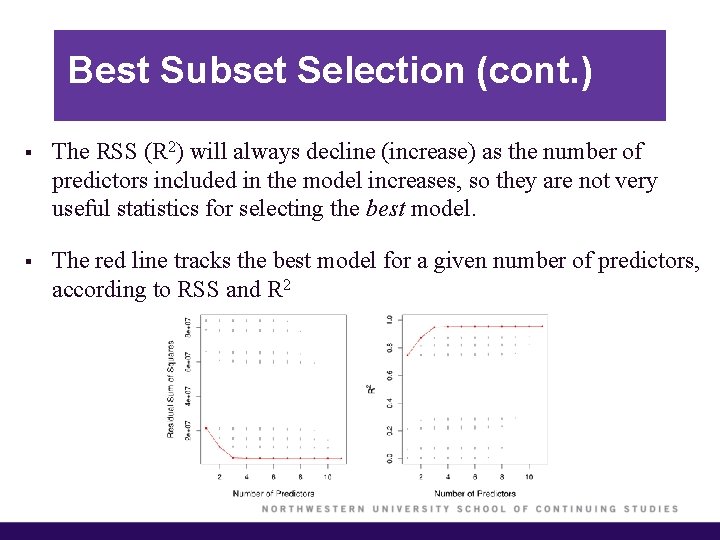
Best Subset Selection (cont. ) § The RSS (R 2) will always decline (increase) as the number of predictors included in the model increases, so they are not very useful statistics for selecting the best model. § The red line tracks the best model for a given number of predictors, according to RSS and R 2

Best Subset Selection (cont. ) § While best subset selection is a simple and conceptually appealing approach, it suffers from computational limitations. § The number of possible models that must be considered grows rapidly as p increases. § Best subset selection becomes computationally infeasible for value of p greater than around 40.

Stepwise Selection § For computational reasons, best subset selection cannot be applied with very large p. § The larger the search space, the higher the chance of finding models that look good on the training data, even though they might not have any predictive power on future data. § An enormous search space can lead to overfitting and high variance of the coefficient estimates.

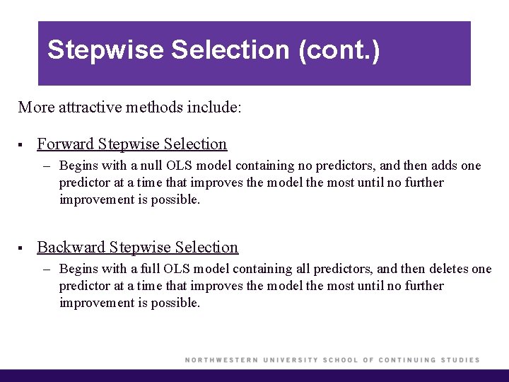
Stepwise Selection (cont. ) More attractive methods include: § Forward Stepwise Selection – Begins with a null OLS model containing no predictors, and then adds one predictor at a time that improves the model the most until no further improvement is possible. § Backward Stepwise Selection – Begins with a full OLS model containing all predictors, and then deletes one predictor at a time that improves the model the most until no further improvement is possible.

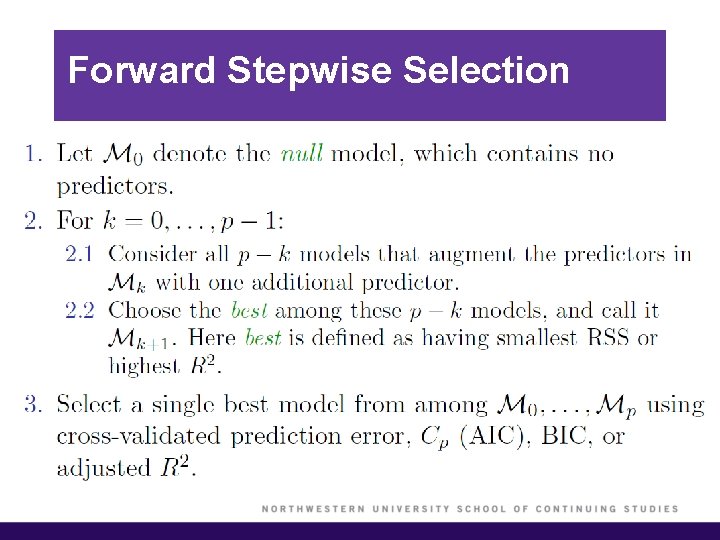
Forward Stepwise Selection

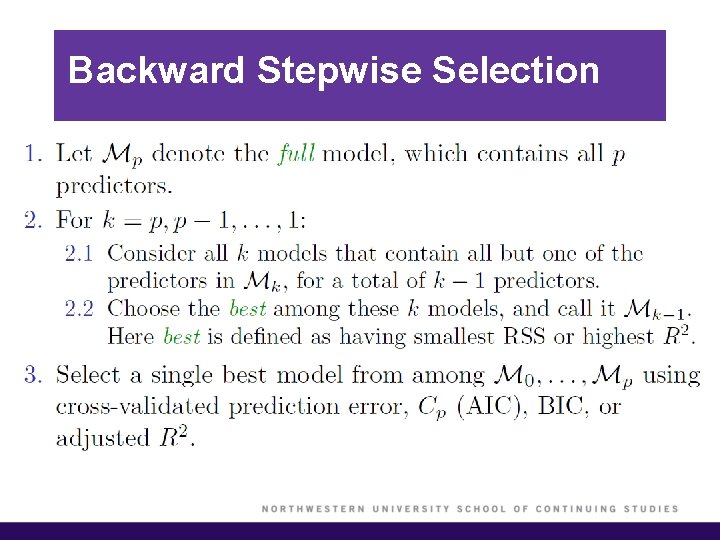
Backward Stepwise Selection

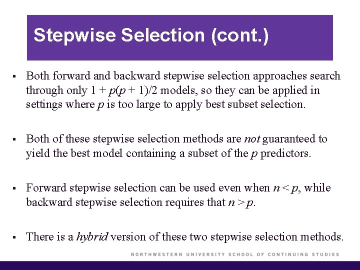
Stepwise Selection (cont. ) § Both forward and backward stepwise selection approaches search through only 1 + p(p + 1)/2 models, so they can be applied in settings where p is too large to apply best subset selection. § Both of these stepwise selection methods are not guaranteed to yield the best model containing a subset of the p predictors. § Forward stepwise selection can be used even when n < p, while backward stepwise selection requires that n > p. § There is a hybrid version of these two stepwise selection methods.

Choosing the Optimal Model § The model containing all the predictors will always have the smallest RSS and the largest R 2, since these quantities are related to the training error. § We wish to choose a model with low test error, not a model with low training error. Recall that training error is usually a poor estimate of test error. § Thus, RSS and R 2 are not suitable for selecting the best model among a collection of models with different numbers of predictors.

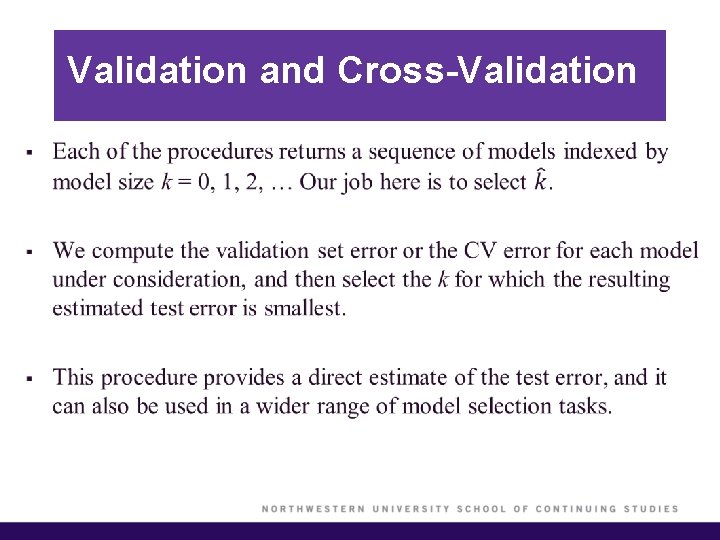
Estimating Test Error 1. We can indirectly estimate test error by making an adjustment to the training error to account for the bias due to overfitting. 2. We can directly estimate the test error, using either a validation set approach or a crossvalidation approach.

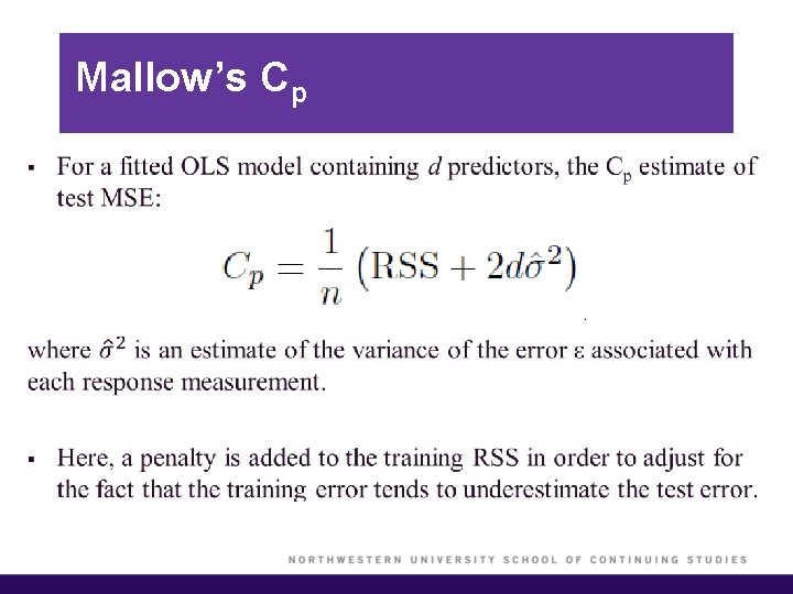
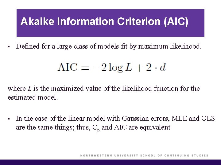
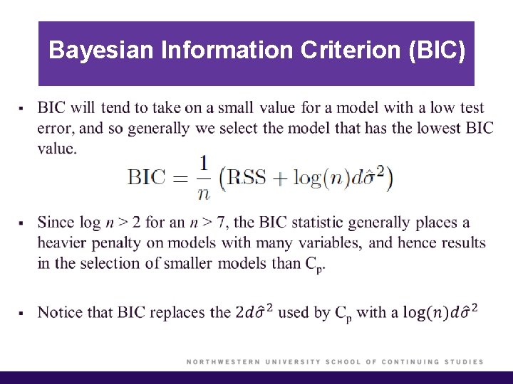
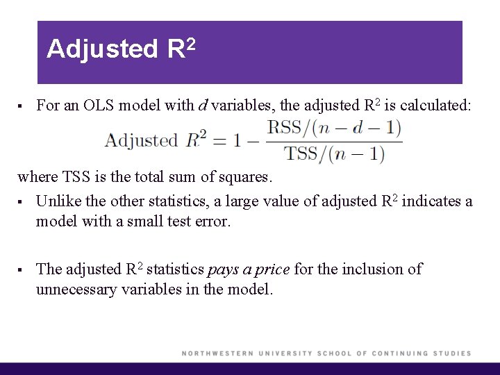
Other Measures of Comparison § To compare different models, we can use other approaches: – Adjusted R 2 – AIC (Akaike information criterion) – BIC (Bayesian information criterion) – Mallow’s Cp (equivalent to AIC for linear regression) § These techniques adjust the training error for the model size, and can be used to select among a set of models with different numbers of variables. § These methods add penalty to RSS for the number of predictors in the model.

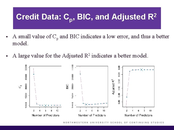
Credit Data: Cp, BIC, and Adjusted R 2 § A small value of Cp and BIC indicates a low error, and thus a better model. § A large value for the Adjusted R 2 indicates a better model.

Mallow’s Cp §

Akaike Information Criterion (AIC) § Defined for a large class of models fit by maximum likelihood. where L is the maximized value of the likelihood function for the estimated model. § In the case of the linear model with Gaussian errors, MLE and OLS are the same things; thus, Cp and AIC are equivalent.

Bayesian Information Criterion (BIC) §

Adjusted R 2 § For an OLS model with d variables, the adjusted R 2 is calculated: where TSS is the total sum of squares. § Unlike the other statistics, a large value of adjusted R 2 indicates a model with a small test error. § The adjusted R 2 statistics pays a price for the inclusion of unnecessary variables in the model.

Validation and Cross-Validation §

Shrinkage (Regularization) Methods § The subset selection methods use OLS to fit a linear model that contains a subset of the predictors. § As an alternative, we can fit a model containing all p predictors using a technique that constrains or regularizes the coefficient estimates (i. e. shrinks the coefficient estimates towards zero). § It may not be immediately obvious why such a constraint should improve the fit, but it turns out that shrinking the coefficient estimates can significantly reduce their variance.

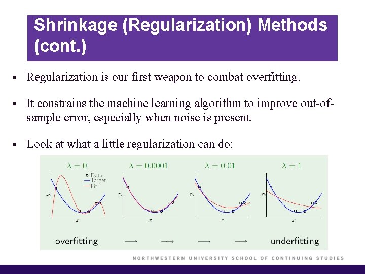
Shrinkage (Regularization) Methods (cont. ) § Regularization is our first weapon to combat overfitting. § It constrains the machine learning algorithm to improve out-ofsample error, especially when noise is present. § Look at what a little regularization can do:

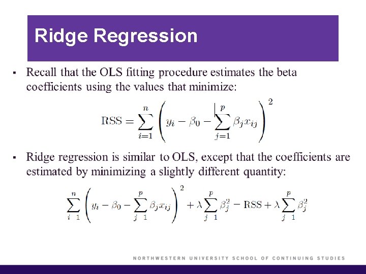
Ridge Regression §

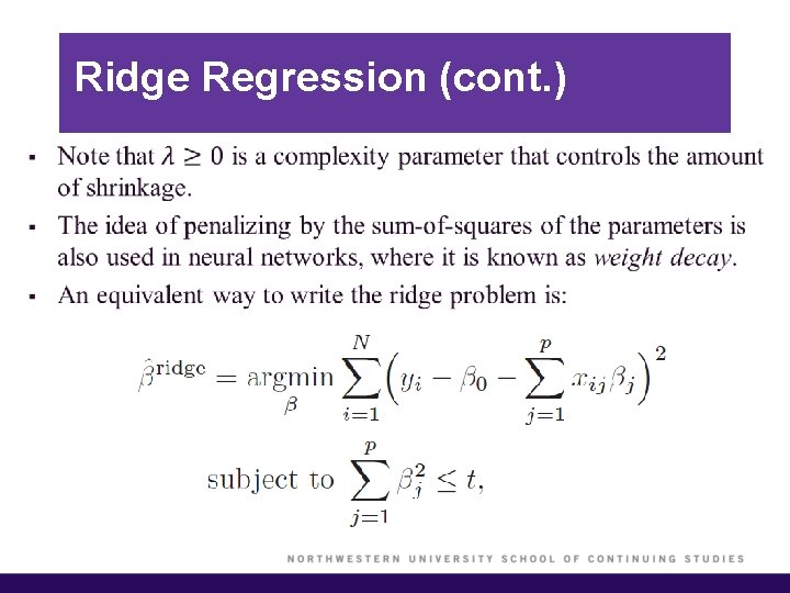
Ridge Regression (cont. ) §

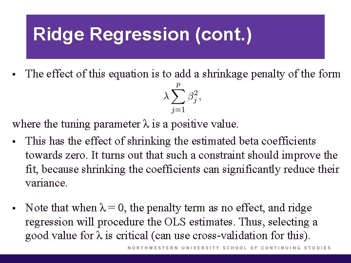
Ridge Regression (cont. ) § The effect of this equation is to add a shrinkage penalty of the form where the tuning parameter λ is a positive value. § This has the effect of shrinking the estimated beta coefficients towards zero. It turns out that such a constraint should improve the fit, because shrinking the coefficients can significantly reduce their variance. § Note that when λ = 0, the penalty term as no effect, and ridge regression will procedure the OLS estimates. Thus, selecting a good value for λ is critical (can use cross-validation for this).

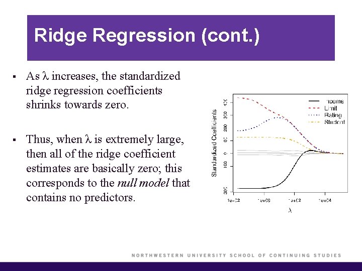
Ridge Regression (cont. ) § As λ increases, the standardized ridge regression coefficients shrinks towards zero. § Thus, when λ is extremely large, then all of the ridge coefficient estimates are basically zero; this corresponds to the null model that contains no predictors.

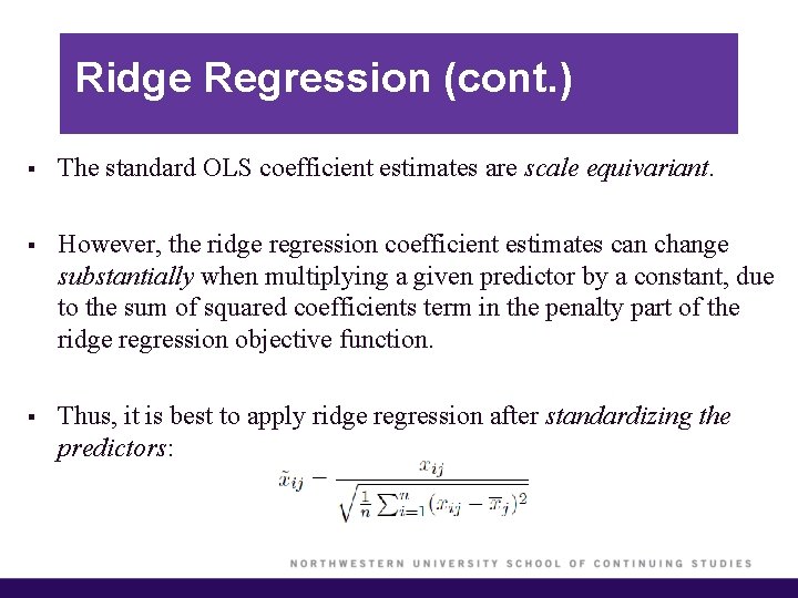
Ridge Regression (cont. ) § The standard OLS coefficient estimates are scale equivariant. § However, the ridge regression coefficient estimates can change substantially when multiplying a given predictor by a constant, due to the sum of squared coefficients term in the penalty part of the ridge regression objective function. § Thus, it is best to apply ridge regression after standardizing the predictors:

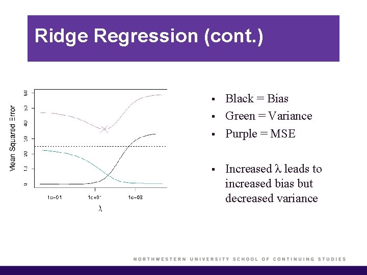
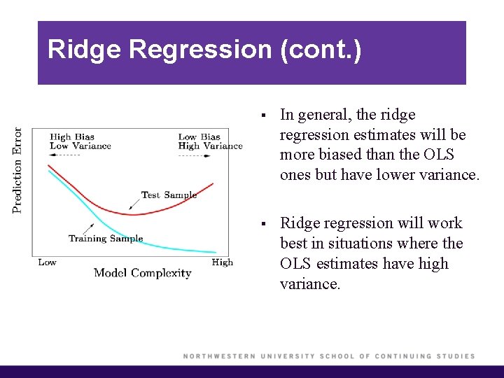
Ridge Regression (cont. ) § It turns out that the OLS estimates generally have low bias but can be highly variable. In particular when n and p are of similar size or when n < p, then the OLS estimates will be extremely variable § The penalty term makes the ridge regression estimates biased but can also substantially reduce variance § As a result, there is a bias/variance trade-off.

Ridge Regression (cont. ) § § Black = Bias Green = Variance Purple = MSE Increased λ leads to increased bias but decreased variance

Ridge Regression (cont. ) § In general, the ridge regression estimates will be more biased than the OLS ones but have lower variance. § Ridge regression will work best in situations where the OLS estimates have high variance.

Ridge Regression (cont. ) Computational Advantages of Ridge Regression § If p is large, then using the best subset selection approach requires searching through enormous numbers of possible models. § With ridge regression, for any given λ we only need to fit one model and the computations turn out to be very simple. § Ridge regression can even be used when p > n, a situation where OLS fails completely (i. e. OLS estimates do not even have a unique solution).

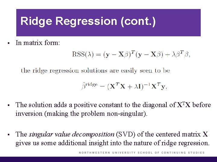
Ridge Regression (cont. ) § In matrix form: § The solution adds a positive constant to the diagonal of XTX before inversion (making the problem non-singular). § The singular value decomposition (SVD) of the centered matrix X gives us some additional insight into the nature of ridge regression.

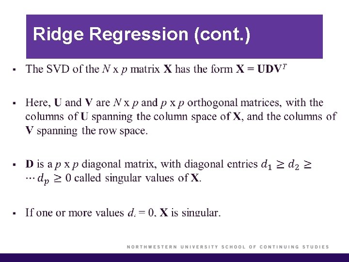
Ridge Regression (cont. ) §

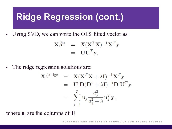
Ridge Regression (cont. ) § Using SVD, we can write the OLS fitted vector as: § The ridge regression solutions are: where uj are the columns of U.

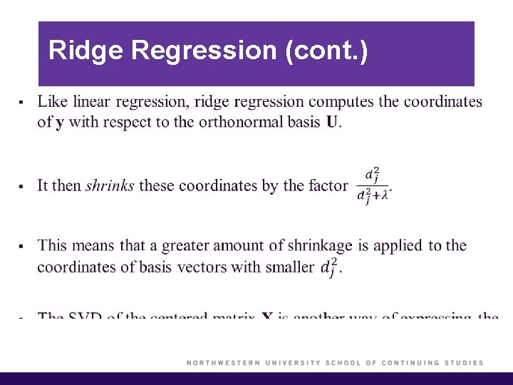
Ridge Regression (cont. ) §

Ridge Regression (cont. ) § Thus, we have XTX = VD 2 VT, which is the eigen decomposition of XTX. § The eigenvectors vj (columns of V) are also called the principal components directions of X. § The first principal component direction v 1 has the property that z 1 = Xv 1 has the largest sample variance amongst all normalized linear combinations of the columns of X. § The small singular values dj correspond to directions in the column space of X having small variance, and ridge regression shrinks these directions the most.

The Lasso § One significant problem of ridge regression is that the penalty term will never force any of the coefficients to be exactly zero. § Thus, the final model will include all p predictors, which creates a challenge in model interpretation § A more modern machine learning alternative is the lasso. § The lasso works in a similar way to ridge regression, except it uses a different penalty term that shrinks some of the coefficients exactly to zero.

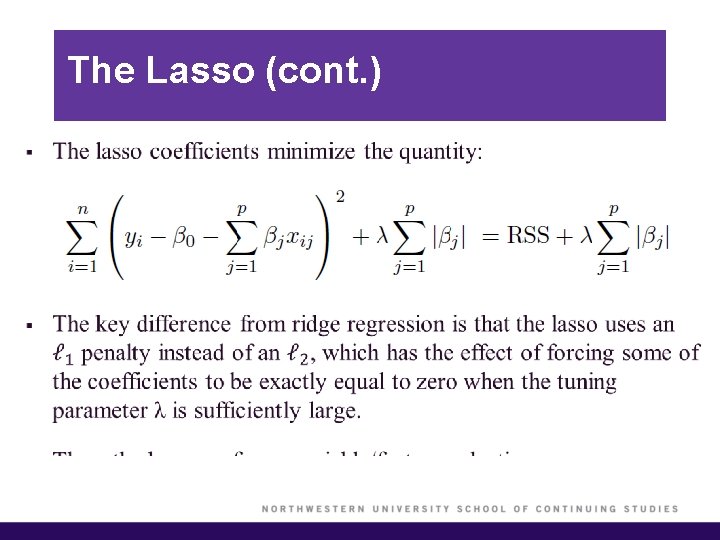
The Lasso (cont. ) §

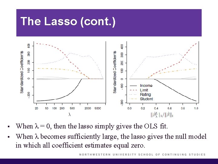
The Lasso (cont. ) § § When λ = 0, then the lasso simply gives the OLS fit. When λ becomes sufficiently large, the lasso gives the null model in which all coefficient estimates equal zero.

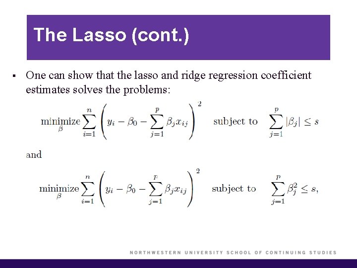
The Lasso (cont. ) § One can show that the lasso and ridge regression coefficient estimates solves the problems:

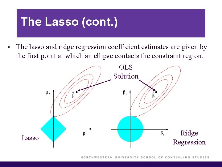
The Lasso (cont. ) § The lasso and ridge regression coefficient estimates are given by the first point at which an ellipse contacts the constraint region. OLS Solution Lasso Ridge Regression

Lasso vs. Ridge Regression § The lasso has a major advantage over ridge regression, in that it produces simpler and more interpretable models that involved only a subset of predictors. § The lasso leads to qualitatively similar behavior to ridge regression, in that as λ increases, the variance decreases and the bias increases. § The lasso can generate more accurate predictions compared to ridge regression. § Cross-validation can be used in order to determine which approach is better on a particular data set.

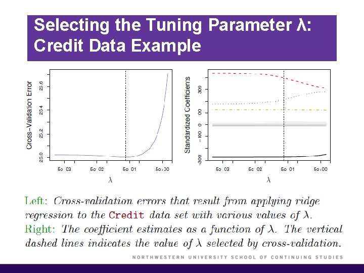
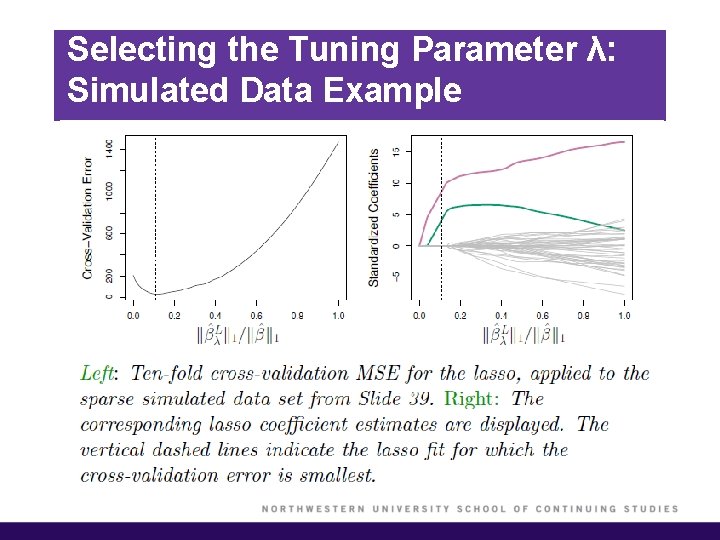
Selecting the Tuning Parameter λ § As for subset selection, for ridge regression and lasso we require a method to determine which of the models under consideration in best; thus, we required a method selecting a value for the tuning parameter λ or equivalently, the value of the constraint s. § Select a grid of potential values; use cross-validation to estimate the error rate on test data (for each value of λ) and select the value that gives the smallest error rate. § Finally, the model is re-fit using all of the variable observations and the selected value of the tuning parameter λ.

Selecting the Tuning Parameter λ: Credit Data Example

Selecting the Tuning Parameter λ: Simulated Data Example

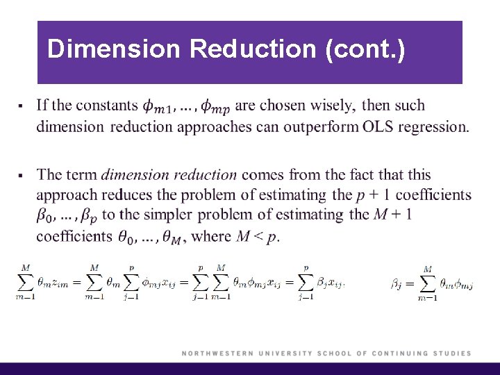
Dimension Reduction § The methods we have discussed so far have involved fitting linear regression models, via OLS or a shrunken approach, using the original predictors. § We now explore a class of approaches that transform the predictors and then fit an OLS model using the transformed variables. § We refer to these techniques as dimension reduction methods.

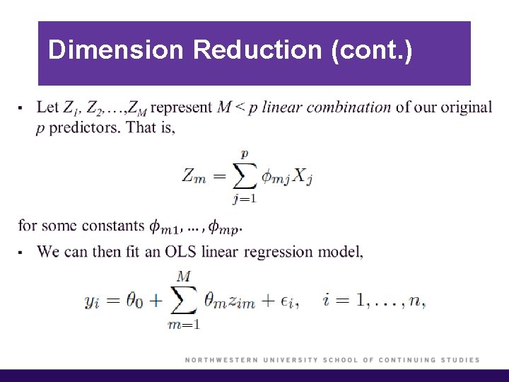
Dimension Reduction (cont. ) §

Dimension Reduction (cont. ) §

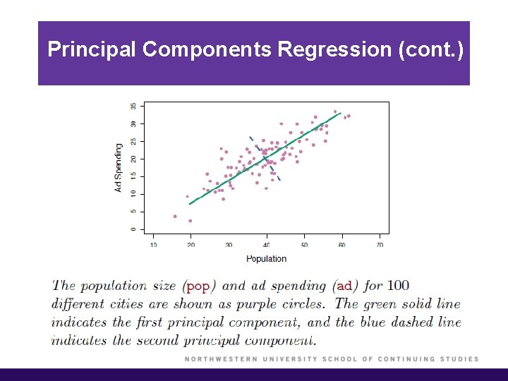
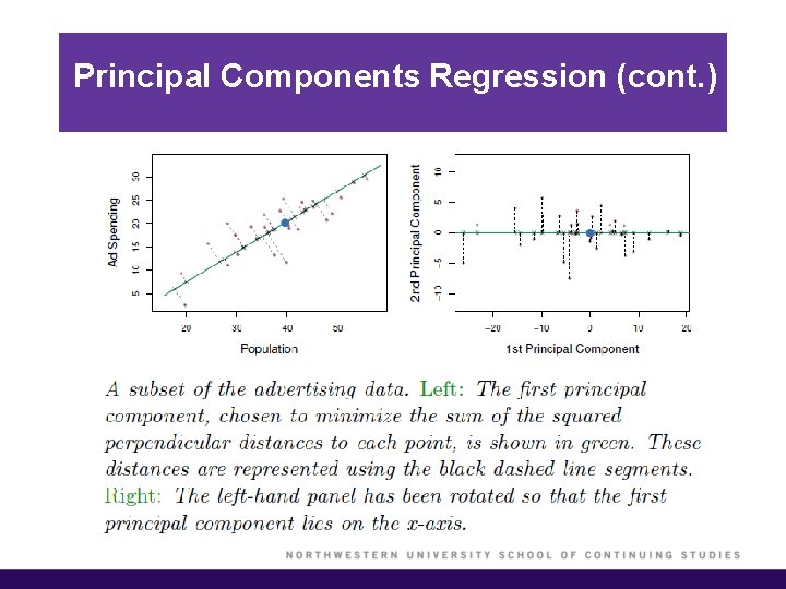
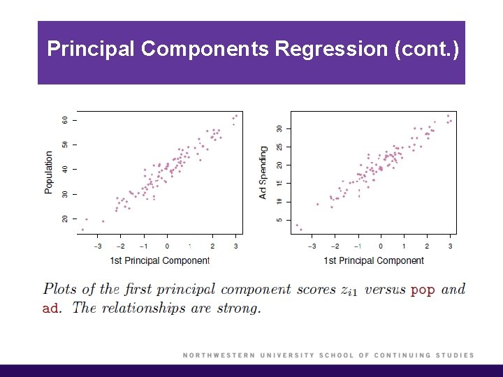
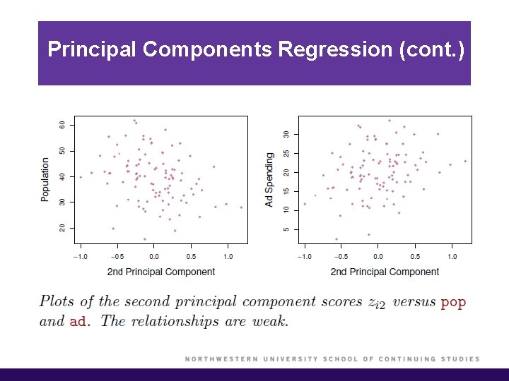
Principal Components Regression § Here, we apply principal components analysis (PCA) to define the linear combinations of the predictors, for use in the regression. § The first principal component is that (normalized) linear combination of the variables with the largest variances. § The second principal component has largest variance, subject to being uncorrelated with the first…. etc. § Thus, with many correlated variables, we replace them with a small set of principal components that capture their joint variation.

Principal Components Regression (cont. ) § The principal components regression (PCR) approach involves constructing the first M principal components, and then using these components as the predictors in an OLS linear regression model. § The key idea is that often a small number of principal components suffice to explain most of the variability in the data, as well as the relationship with the response. § We assume that the directions in which X 1, …, Xp show the most variation are the directions that are associated with Y. § When performing PCR, predictors should be standardized prior to generating the principal components.

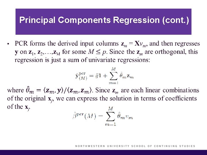
Principal Components Regression (cont. ) §

Principal Components Regression (cont. ) § By manually setting the projection onto the principal component directions with small eigenvalues set to 0 (i. e. , only keeping the large ones), dimension reduction is achieved. § PCR is very similar to ridge regression in a certain sense. § Ridge regression can be viewed conceptually as projecting the y vector onto the principal component directions and then shrinking the projection on each principal component direction.

Principal Components Regression (cont. ) § The amount of shrinkage depends on the variance of that principal component. § Ridge regression shrinks everything, but it never shrinks anything to zero. § By contrast, PCR either does not shrink a component at all or shrinks it to zero.

Principal Components Regression (cont. )

Principal Components Regression (cont. )

Principal Components Regression (cont. )

Principal Components Regression (cont. )

Principal Components Regression (cont. )

Principal Components Regression (cont. )

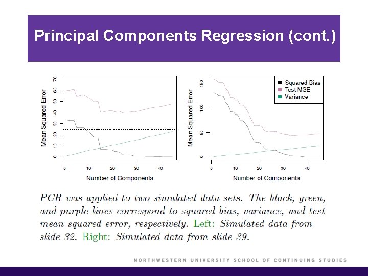
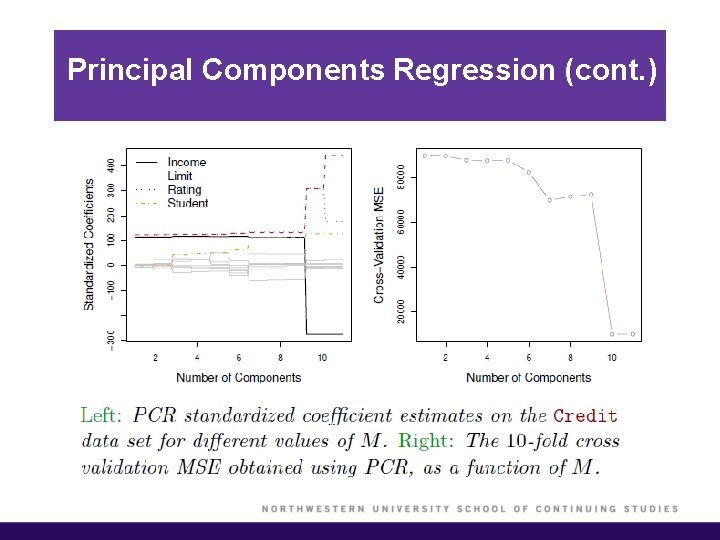
Principal Components Regression (cont. ) § As more principal components are used in the regression model, the bias decreases but the variance increases. § PCR will tend to do well in cases when the first few principal components are sufficient to capture most of the variation in the predictors as well as the relationship with the response. § We note that even though PCR provides a simple way to perform regression using M < p predictors, it is not a feature selection method. § In PCR, the number of principal components is typically chosen by cross-validation.

Partial Least Squares § PCR identifies linear combinations, or directions, that best represents the predictors. § These directions are identified is an unsupervised way, since the response Y is not used to help determine the principal component directions. § That is, the response does not supervise the identification of the principal components. § PCR suffers from a potentially serious drawback: there is no guarantee that the directions that best explain the predictors will also be the best directions to use for predicting the response.

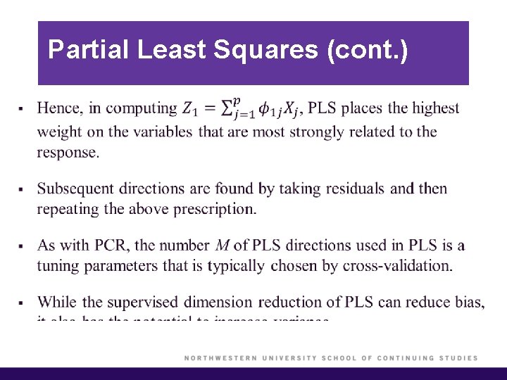
Partial Least Squares (cont. ) § Like PCR, partial least squares (PLS) is a dimension reduction method, which first identifies a new set of features Z 1, …, ZM that are linear combinations of the original features. § Then PLS fits an OLS linear model using these M new features. § Unlike PCR, PLS identifies these new features in a supervised way; PLS makes use of the response Y in order to identify new features that not only approximate the old features well, but also that are related to the response. § The PLS approach attempts to find directions that help explain both the response and the predictors.

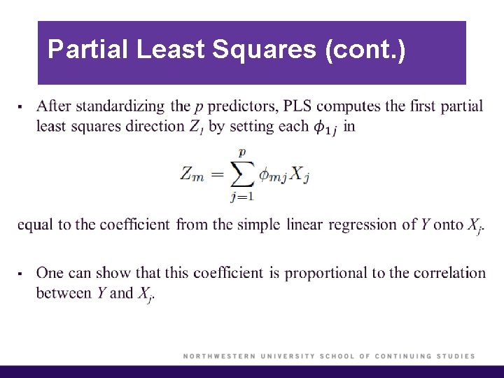
Partial Least Squares (cont. ) §

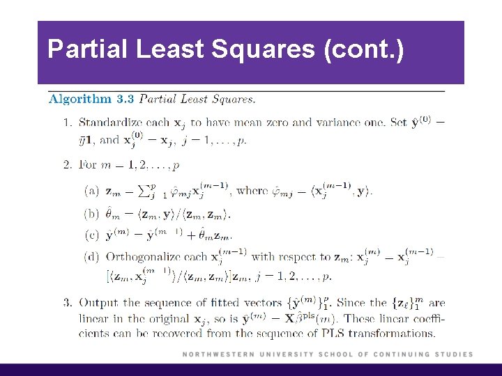
Partial Least Squares (cont. ) §

Partial Least Squares (cont. )

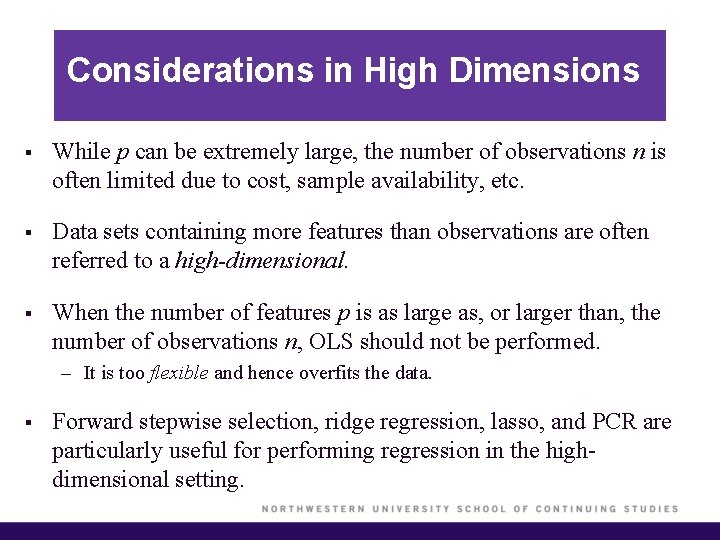
Considerations in High Dimensions § While p can be extremely large, the number of observations n is often limited due to cost, sample availability, etc. § Data sets containing more features than observations are often referred to a high-dimensional. § When the number of features p is as large as, or larger than, the number of observations n, OLS should not be performed. – It is too flexible and hence overfits the data. § Forward stepwise selection, ridge regression, lasso, and PCR are particularly useful for performing regression in the highdimensional setting.

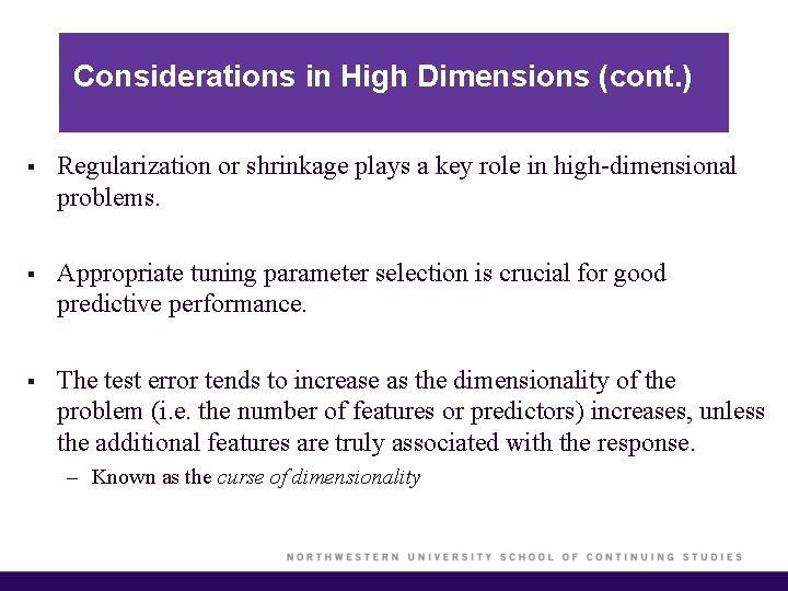
Considerations in High Dimensions (cont. ) § Regularization or shrinkage plays a key role in high-dimensional problems. § Appropriate tuning parameter selection is crucial for good predictive performance. § The test error tends to increase as the dimensionality of the problem (i. e. the number of features or predictors) increases, unless the additional features are truly associated with the response. – Known as the curse of dimensionality

Considerations in High Dimensions (cont. ) § Curse of dimensionality – Adding additional signal features that are truly associated with the response will improve the fitted model, in the sense of leading to a reduction in test set error. – Adding noise features that are not truly associated with the response will lead to a deterioration in the fitted model, and consequently an increased test set error. § Noise features increase the dimensionality of the problem, exacerbating the risk of overfitting without any potential upside in terms of improved test set error.

Considerations in High Dimensions (cont. ) § In the high-dimensional setting, the multicollinearity problem is extreme: any variable in the model can be written as a linear combination of all of the other variables in the models. § It is also important to be particularly careful in reporting errors and measures of model fit in the high-dimensional setting. § One should never use sum of squared errors, p-values, R 2 statistics, or other traditional measures of model fit on the training data as evidence of good model fit in the high-dimensional setting. § It is important to report results on an independent test set, or crossvalidation errors.

Summary § § § Best subset selection and stepwise selection methods. Estimate test error by adjusting training error to account for bias due to overfitting. Estimate test error using validation set approach and cross-validation approach. Ridge regression and the lasso as shrinkage (regularization) methods. Principal components regression and partial least squares. Considerations for high-dimensional settings.