PREDICT 422 Practical Machine Learning Module 7 Perceptron

PREDICT 422: Practical Machine Learning Module 7: Perceptron Learning Algorithm and Artificial Neural Networks Lecturer: Nathan Bastian, Section: XXX

Assignment § Reading: None § Activity: Begin Course Project

References § The Elements of Statistical Learning (2009), by T. Hastie, R. Tibshirani, and J. Friedman. § Machine Learning: A Probabilistic Perspective (2012), by K. Murphy

Lesson Goals: § Understand the basic concepts of one of the oldest machine learning methods, the perceptron learning algorithm, for the problem of separating hyperplanes. § Understand artificial neural networks and the back-propagation algorithm for both regression and classification problems.

Separating Hyperplanes § We seek to construct linear decision boundaries that explicitly try to separate the data into different classes as well as possible. § We have seen that LDA and logistic regression both estimate linear decision boundaries in similar but slightly different ways. § Even when the training data can be perfectly separated by hyperplanes, LDA or other linear methods developed under a statistical framework may not achieve perfect separation. § Instead of using a probabilistic argument to estimate parameters, here we consider a geometric argument.

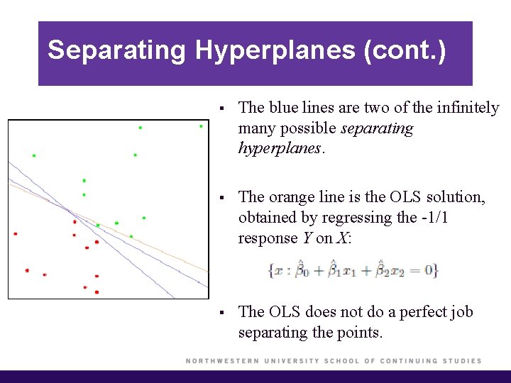
Separating Hyperplanes (cont. ) § The blue lines are two of the infinitely many possible separating hyperplanes. § The orange line is the OLS solution, obtained by regressing the -1/1 response Y on X: § The OLS does not do a perfect job separating the points.

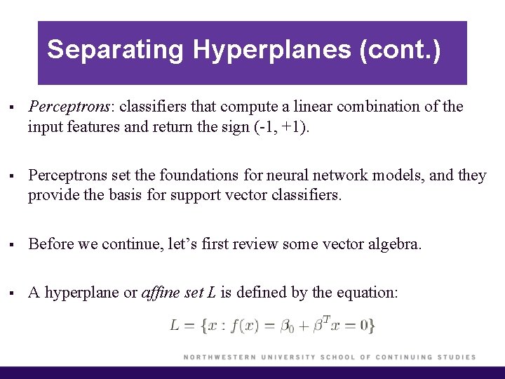
Separating Hyperplanes (cont. ) § Perceptrons: classifiers that compute a linear combination of the input features and return the sign (-1, +1). § Perceptrons set the foundations for neural network models, and they provide the basis for support vector classifiers. § Before we continue, let’s first review some vector algebra. § A hyperplane or affine set L is defined by the equation:

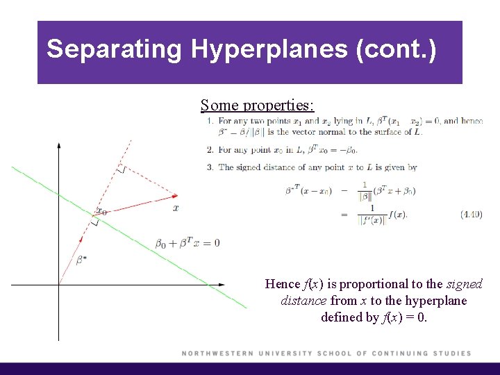
Separating Hyperplanes (cont. ) Some properties: Hence f(x) is proportional to the signed distance from x to the hyperplane defined by f(x) = 0.

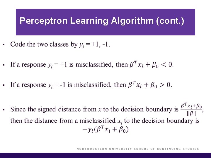
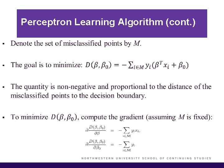
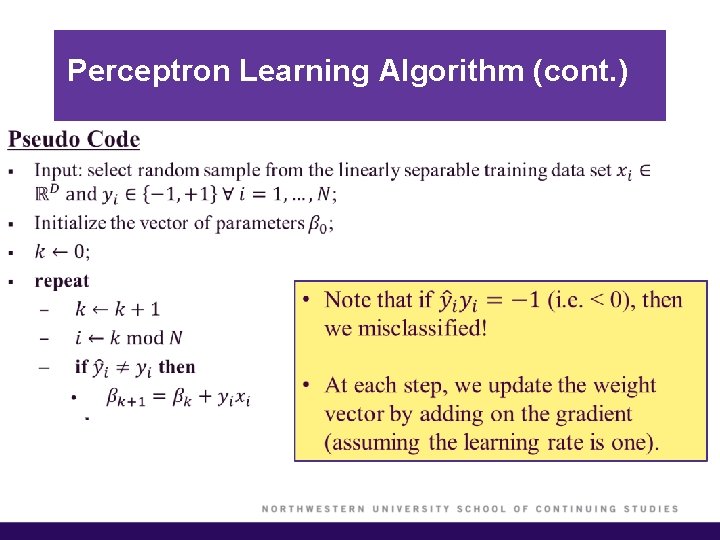
Perceptron Learning Algorithm § One of the older approaches to this problem of finding a separating hyperplane in the machine learning literature is called the perceptron learning algorithm, developed by Frank Rosenblatt in 1956. § Goal: The algorithm tries to find a separating hyperplane by minimizing the distance of misclassified points to the decision boundary. § The algorithm starts with an initial guess as to the separating plane’s parameters and then updates that guess when it makes mistakes.

Perceptron Learning Algorithm (cont. ) §

Perceptron Learning Algorithm (cont. ) §

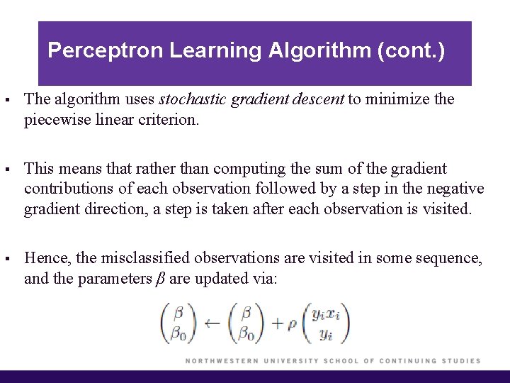
Perceptron Learning Algorithm (cont. ) § The algorithm uses stochastic gradient descent to minimize the piecewise linear criterion. § This means that rather than computing the sum of the gradient contributions of each observation followed by a step in the negative gradient direction, a step is taken after each observation is visited. § Hence, the misclassified observations are visited in some sequence, and the parameters β are updated via:

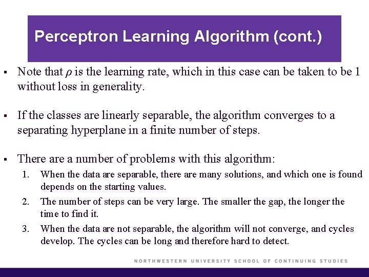
Perceptron Learning Algorithm (cont. ) § Note that ρ is the learning rate, which in this case can be taken to be 1 without loss in generality. § If the classes are linearly separable, the algorithm converges to a separating hyperplane in a finite number of steps. § There a number of problems with this algorithm: 1. 2. 3. When the data are separable, there are many solutions, and which one is found depends on the starting values. The number of steps can be very large. The smaller the gap, the longer the time to find it. When the data are not separable, the algorithm will not converge, and cycles develop. The cycles can be long and therefore hard to detect.

Perceptron Learning Algorithm (cont. ) §

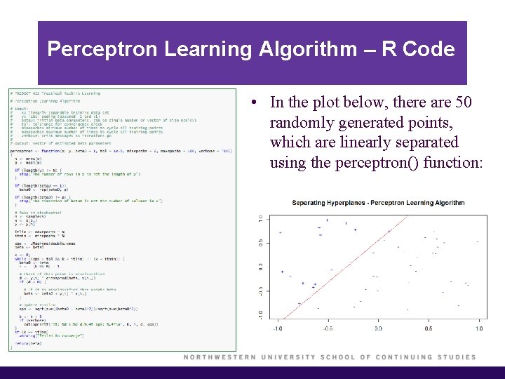
Perceptron Learning Algorithm – R Code • In the plot below, there are 50 randomly generated points, which are linearly separated using the perceptron() function:

Artificial Neural Networks § The central idea of artificial neural networks (ANN) is to extract linear combinations of the inputs as derived features, and then model the target as a nonlinear function of these features. § This machine learning method originated as an algorithm trying to mimic neurons and the brain. § The brain has extraordinary computational power to represent and interpret complex environments. § ANN attempts to capture this mode of computation.

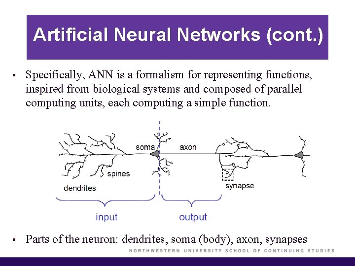
Artificial Neural Networks (cont. ) § Specifically, ANN is a formalism for representing functions, inspired from biological systems and composed of parallel computing units, each computing a simple function. § Parts of the neuron: dendrites, soma (body), axon, synapses

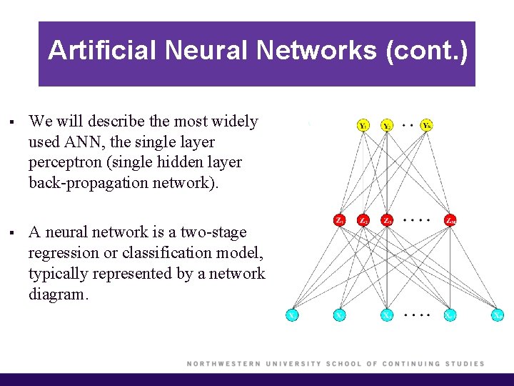
Artificial Neural Networks (cont. ) § We will describe the most widely used ANN, the single layer perceptron (single hidden layer back-propagation network). § A neural network is a two-stage regression or classification model, typically represented by a network diagram.

Artificial Neural Networks (cont. ) § For regression, typically K = 1 and there is only one output unit Y 1 at the top of the network diagram. § These networks, however, can handle multiple quantitative responses in a seamless fashion. § For K-classification, there are K units at the top of the network diagram, with the kth unit modeling the probability of class k. § There are K target measurements Yk, k = 1, …, K, each being coded as a 0 – 1 variable for the kth class.

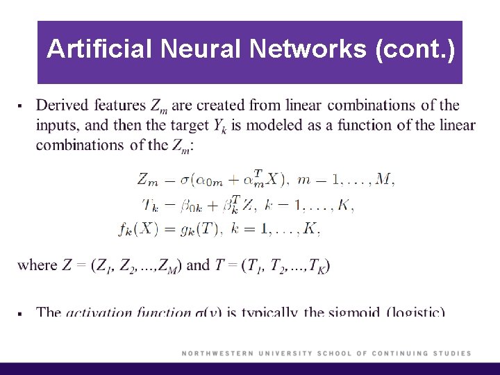
Artificial Neural Networks (cont. ) §

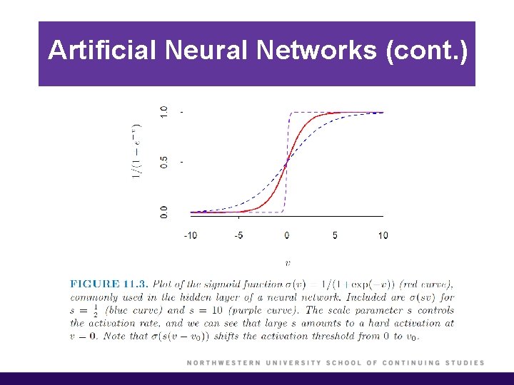
Artificial Neural Networks (cont. )

Artificial Neural Networks (cont. ) §

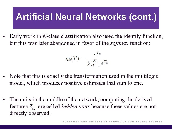
Artificial Neural Networks (cont. ) § Early work in K-classification also used the identity function, but this was later abandoned in favor of the softmax function: § Note that this is exactly the transformation used in the multilogit model, which produces positive estimates that sum to one. § The units in the middle of the network, computing the derived features Zm, are called hidden units because these values are not directly observed.

Artificial Neural Networks (cont. ) § We can think of the Zm as a basis expansion of the original inputs X; the neural network is then a standard linear model, or linear multilogit model, using these transformations as inputs. § However, the parameters of the basis functions are learned from the data, which is an important enhancement over the basis expansion techniques. § Notice that if σ is the identity function, then the entire model collapses to a linear model in the inputs.

Artificial Neural Networks (cont. ) § Thus, a neural network can be though of as a nonlinear generalization of the linear model, both for regression and classification. § By introducing the nonlinear transformation σ, it greatly enlarges the class of linear models. § In general, there can be more than one hidden layer. § The neural network model has unknown parameters, often called weights.

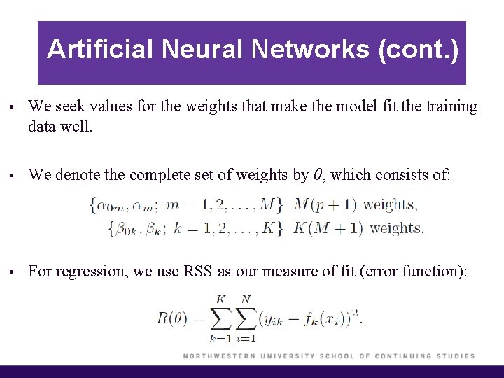
Artificial Neural Networks (cont. ) § We seek values for the weights that make the model fit the training data well. § We denote the complete set of weights by θ, which consists of: § For regression, we use RSS as our measure of fit (error function):

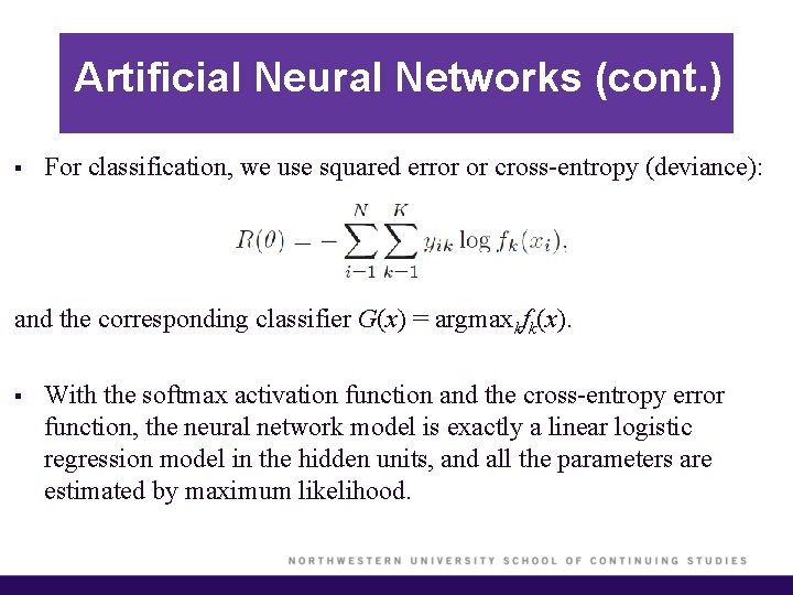
Artificial Neural Networks (cont. ) § For classification, we use squared error or cross-entropy (deviance): and the corresponding classifier G(x) = argmaxkfk(x). § With the softmax activation function and the cross-entropy error function, the neural network model is exactly a linear logistic regression model in the hidden units, and all the parameters are estimated by maximum likelihood.

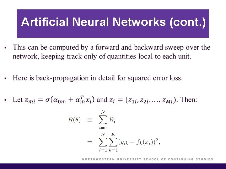
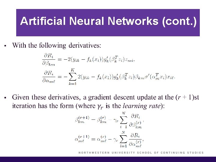
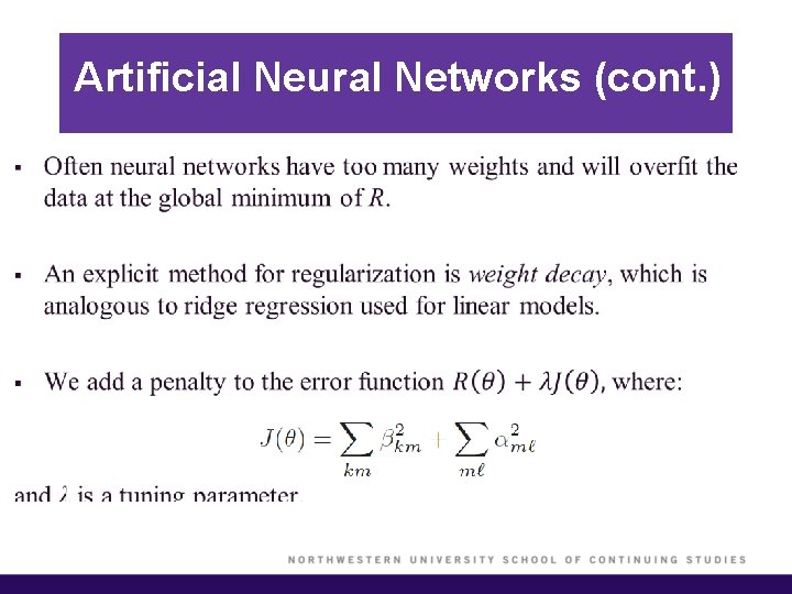
Artificial Neural Networks (cont. ) § Typically, we do not want the global minimizer R(θ), as this is likely to be an overfit solution. § Instead, some regularization is need; this is achieved directly through a penalty term, or indirectly by early stopping. § The generic approach to minimizing R(θ) is by gradient descent, called back-propagation in this setting. § The gradient can be easily derived using the chain rule for differentiation.

Artificial Neural Networks (cont. ) §

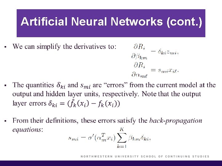
Artificial Neural Networks (cont. ) §

Artificial Neural Networks (cont. ) §

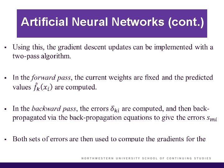
Artificial Neural Networks (cont. ) §

Artificial Neural Networks (cont. ) § This two-pass procedure is what is known as back-propagation. § It has also been called the delta rule. § The computational components for cross-entropy have the same form as those for the sum of squares function. § The advantage of back-propagation are its simple, local nature. In the back-propagation algorithm, each hidden unit passes and receives information only to and from units that share a connection.

Artificial Neural Networks (cont. ) § Usually starting values for weights are chosen to be random values near zero. § Hence, the model starts out nearly linear and becomes nonlinear as the weights increase. § Use of exact zero weights leads to zero derivatives and perfect symmetry, and the algorithm never moves. § Starting instead with large weights often leads to poor solutions.

Artificial Neural Networks (cont. ) §

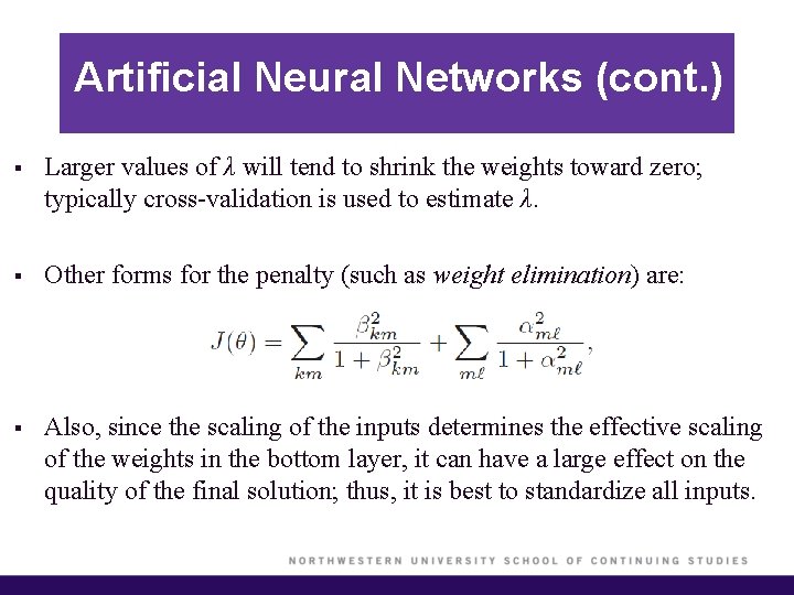
Artificial Neural Networks (cont. ) § Larger values of λ will tend to shrink the weights toward zero; typically cross-validation is used to estimate λ. § Other forms for the penalty (such as weight elimination) are: § Also, since the scaling of the inputs determines the effective scaling of the weights in the bottom layer, it can have a large effect on the quality of the final solution; thus, it is best to standardize all inputs.

Artificial Neural Networks (cont. ) § Generally, it is better to have too many hidden units than too few. § With too few hidden units, the model might not have enough flexibility to capture the nonlinearities in the data. § With too many hidden units, the extra weights can be shrunk toward zero if appropriate regularization is used. § Typically the number of hidden units is somewhere in the range of 5 to 100, with the number increasing with the number of inputs and number of training cases.

Artificial Neural Networks (cont. ) § The error function is nonconvex, possessing many local minima, so one must try a number of random starting configurations and the choose the solution giving the lowest error. § Probably a better approach is to use the average predictions over the collection of networks as the final prediction. § Another approach is via bagging, which averages the predictions of networks training from randomly perturbed version of the training data.

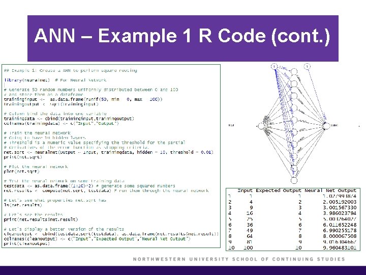
ANN – Example 1 R Code § In this first example, we use the R library “neuralnet” to train and build a neural network that is able to take a number and calculate the square root. § The ANN will take a single input (the number you want square rooting) and produce a single output (the square root of the input). § The ANN will contain 10 hidden neurons to be trained within each layer. § The ANN does a reasonable job at finding the square root!

ANN – Example 1 R Code (cont. )

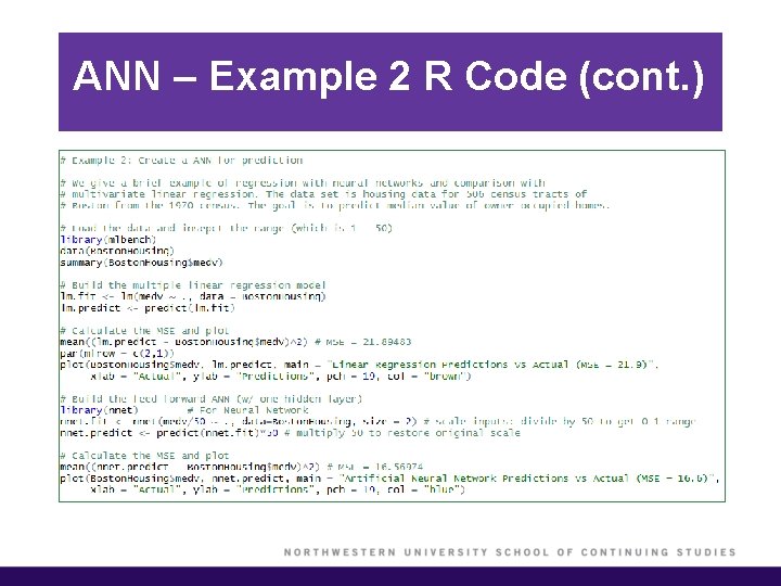
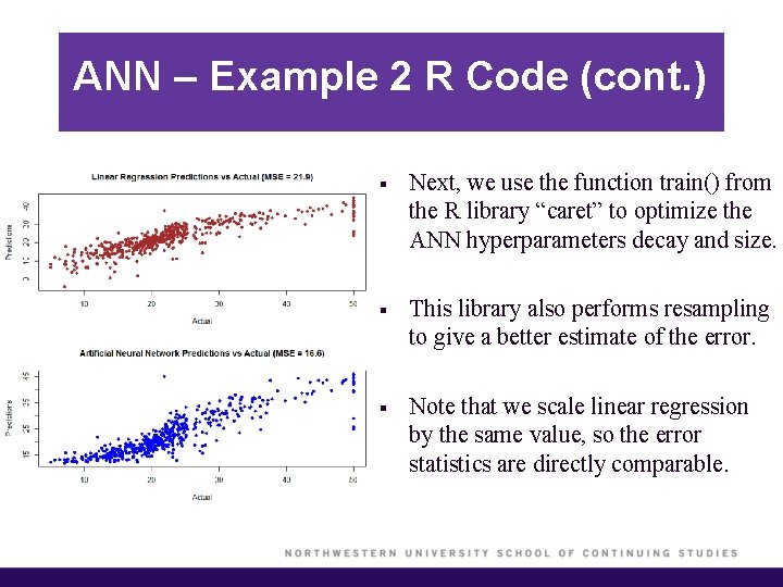
ANN – Example 2 R Code § In this second example, we use the R library “nnet” to train and build a neural network that is able to predict median value of owneroccupied homes. § This example of regression with neural networks is compared with multiple linear regression. § The data set is housing data for 506 census tracts of Boston from the 1970 census. § We see that the ANN outperforms linear regression in terms of lower MSE.

ANN – Example 2 R Code (cont. )

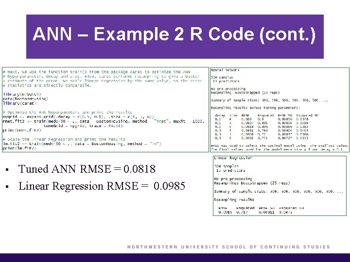
ANN – Example 2 R Code (cont. ) § Next, we use the function train() from the R library “caret” to optimize the ANN hyperparameters decay and size. § This library also performs resampling to give a better estimate of the error. § Note that we scale linear regression by the same value, so the error statistics are directly comparable.

ANN – Example 2 R Code (cont. ) § § Tuned ANN RMSE = 0. 0818 Linear Regression RMSE = 0. 0985

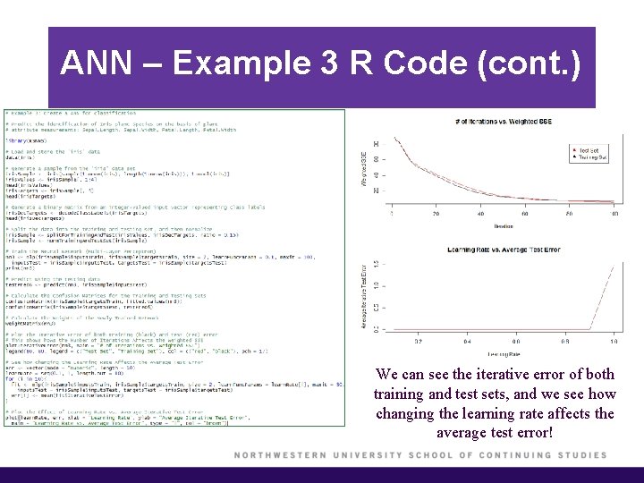
ANN – Example 3 R Code § In this third example, we use the R library “RSNNS” to train and build a neural network that is able to predict the identification of Iris plant Species. § The ANN performs the classification on the basis of plant attribute measurements: Sepal Length, Sepal Width, Petal Length, Petal Width. § This example of classification with neural networks uses the standard back-propagation algorithm.

ANN – Example 3 R Code (cont. ) We can see the iterative error of both training and test sets, and we see how changing the learning rate affects the average test error!

Summary § Perceptron learning algorithm for separating hyperplanes. § Artificial neural networks and the back-propagation algorithm for regression and classification problems.