PREDICT 422 Practical Machine Learning Module 2 Ordinary

Assignment § Reading: Ch. 3 § Activity: Quiz 2, R Lab 2

References § An Introduction to Statistical Learning, with Applications in R (2013), by G.

Lesson Goals: § § § Understand the basic concepts of expectation, variance, and parameter

Overview: Linear Regression § Linear regression is a simple approach to supervised learning, as

Review: Parameter Estimation § In practice, we often seek to select a distribution (model)

OLS Estimation (cont. ) § We illustrate the geometry of OLS fitting, where we

Deciding on Important Variables § Best Subset Selection: we compute the OLS fit for

Overview: Forward Selection § We begin with the null model, a model containing an

Overview: Backward Selection § We begin with all variables in the model. § We

Qualitative Predictors § Some predictors are not quantitative but are qualitative, taking a discrete

Qualitative Predictors (cont. ) § When a qualitative predictor has more than two levels,

Extensions of the Linear Model § Allow for interaction effects. Note that if interaction

Potential Problems § 1. 2. 3. 4. 5. 6. There are several potential problems

Non-linearity of the Data § The linear regression model assumes that there is a

Correlation of Residuals § An important assumption of the linear regression model is that

Non-normality and Non-constant Variance of Residuals § Another important assumption of the linear regression

KNN Regression § K-nearest neighbors (KNN) regression is a non-parametric, flexible approach for performing

KNN Regression (cont. ) § The parametric approach (e. g. linear regression) will outperform

Generalization of the Linear Model Now that we have reviewed linear regression models, we

Summary § § § Review of expectation, variance, and parameter estimation. Basic concepts of

Slides: 50

Download presentation

PREDICT 422: Practical Machine Learning Module 2: Ordinary Least Squares Linear Regression Lecturer: Nathan Bastian, Section: XXX

Assignment § Reading: Ch. 3 § Activity: Quiz 2, R Lab 2

References § An Introduction to Statistical Learning, with Applications in R (2013), by G. James, D. Witten, T. Hastie, and R. Tibshirani. § The Elements of Statistical Learning (2009), by T. Hastie, R. Tibshirani, and J. Friedman. § Learning from Data: A Short Course (2012), by Y. Abu-Mostafa, M. Magdon-Ismail, and H. Lin. § Machine Learning: A Probabilistic Perspective (2012), by K. Murphy

Lesson Goals: § § § Understand the basic concepts of expectation, variance, and parameter estimation. Understand the basic concepts of statistical decision theory. Understand simple and multiple linear regression as a supervised learning algorithm. Understand ordinary least squares estimation for linear regression models. Understand the basic concepts of k-nearest neighbors regression.

Overview: Linear Regression § Linear regression is a simple approach to supervised learning, as it assumes that the dependence of Y on X 1, X 2, …, Xp is linear. § Most modern machine learning approaches can be seen as generalizations or extensions of linear regression. § When augmented with kernels or other forms of basis function expansion (which replace X with some non-linear function of the inputs), it can also model non-linear relationships. § Goal: predict Y from X by f(X)

Review: Expectation §

Review: Expectation (cont. ) §

Review: Variance §

Review: Frequentist Basics §

Review: Parameter Estimation § In practice, we often seek to select a distribution (model) corresponding to our data. § If the model is parameterized by some set of values, then this problem is that of parameter estimation. § In general, we typically use maximum likelihood estimation (MLE) to obtain parameter estimates.

Review: Parameter Estimation (cont. ) §

Statistical Decision Theory §

Statistical Decision Theory (cont. ) §

Linear Regression Model §

Linear Regression Model (cont. ) §

Ordinary Least Squares Estimation §

OLS Estimation (cont. ) §

OLS Estimation (cont. ) § We illustrate the geometry of OLS fitting, where we seek the linear function of X that minimizes the sum of squared residuals from Y. § The predictor function corresponds to a plane (hyper plane) in the 3 D space. § For accurate prediction, hopefully the data will lie close to this hyper plane, but they won’t lie exactly in the hyper plane.

OLS Estimation (cont. ) §

Population vs. OLS Lines §

Accuracy of Coefficient Estimates §

Accuracy of the Model: RSE §

Accuracy of the Model: R 2 §

Two Key Questions §

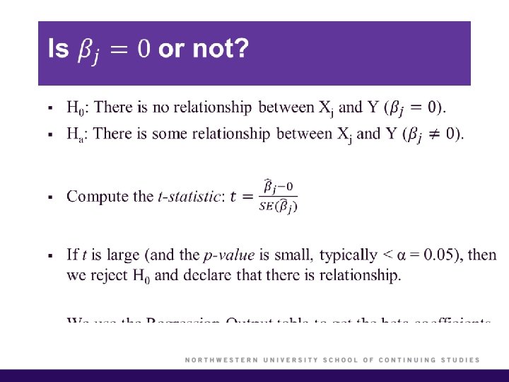
Are all regression coefficients 0? §

Deciding on Important Variables § Best Subset Selection: we compute the OLS fit for all possible subsets of predictors and then choose between them based on some criterion that balances training error with model size. § There are 2 p possible models, so can’t examine them all. § We use an automated approach that searches through a subset of all the models. – Forward Selection – Backward Selection

Overview: Forward Selection § We begin with the null model, a model containing an intercept but no predictors. § We fit p simple linear regressions and add to the null model that variable resulting in the lowest RSS. § We add to that model the variable that results in the lowest RSS amongst all two-variable models. § The algorithm continues until some stopping rule is satisfied (i. e. all remaining variables have a p-value greater than some threshold).

Overview: Backward Selection § We begin with all variables in the model. § We remove the variable with the largest p-value (i. e. least statistically significant). § The new (p – 1)-variable model is fit, and the variable with the largest p-value is removed. § The algorithm continues until a stopping rule is reached.

Qualitative Predictors § Some predictors are not quantitative but are qualitative, taking a discrete set of values. § These are known as categorical variables, which we can code as indicator variables (dummy variables). § Examples: gender, student status, marital status, ethnicity

Qualitative Predictors (cont. ) § When a qualitative predictor has more than two levels, a single dummy variable cannot represent all possible variables. § Thus, there will always be one few dummy variables than the number of levels in the factor. – Factor = Ethnicity – Levels = Asian, Caucasian, African American – # of Dummy Variables = 3 – 1 = 2 § The level with no dummy variable is the baseline.

Qualitative Predictors (cont. ) §

Extensions of the Linear Model § Allow for interaction effects. Note that if interaction is included in the model, all of the main effects should be include as well (even if not statistically significant). § Accommodate non-linear relationships using polynomial regression. For example, you can include transformed versions of the predictors in the model.

Potential Problems § 1. 2. 3. 4. 5. 6. There are several potential problems that may occur when fitting a linear regression model. Non-linearity of the response-predictor relationships. Correlation of residuals. Non-normality and non-constant variance of the residuals. Outliers (refer to Section 3. 3. 3 in text). High-leverage points (refer to Section 3. 3. 3 in text). Collinearity (refer to Section 3. 3. 3 in text).

Non-linearity of the Data § The linear regression model assumes that there is a straight-line relationship between predictors and the response. § If the true relationship is non-linear then conclusions are suspect. § Examine the residual plots, as strong patterns (U-shape) in the residuals indicate non-linearity in the data. § If there are non-linear associations in the data, then use nonlinear transformations of the predictors (e. g. log X).

Correlation of Residuals § An important assumption of the linear regression model is that the residuals are uncorrelated. § If there is correlation among the residuals (Durbin-Watson test), then the estimated standard errors will tend to underestimate the true standard errors – this makes the CIs and PIs narrower than they should be. § These correlations frequently occur in the context of time series data, so consider employing time series analysis methods (such ARIMA, etc. ).

Non-normality and Non-constant Variance of Residuals § Another important assumption of the linear regression model is that the residuals are normally distributed and have constant variance across all levels of X. § If the residuals are not normally distributed (Anderson-Darling test), you can perform a Box-Cox transformation on the response Y. § If there is heteroscedasticity (Breusch-Pagan, Modified Levene, or Special White’s tests), then you can consider transforming the response Y. If this doesn’t fix the problem, consider computing robust standard errors or conduct weighted least squares regression.

KNN Regression § K-nearest neighbors (KNN) regression is a non-parametric, flexible approach for performing regression. § It is closely related to the KNN classifier discussed last week in Module 1. § To predict Y for a given value of X, consider the k closest points to X in the training data and take the average of the responses. § If k is small, then KNN is more flexible than linear regression; it will have low bias but high variance.

KNN Regression (cont. ) § The parametric approach (e. g. linear regression) will outperform the non-parametric approach (e. g. KNN regression) if the parametric form that has been selected is close to the true form of f. § Here, linear regression achieves a lower test MSE than does KNN regression, since f(X) is in fact linear.

Generalization of the Linear Model Now that we have reviewed linear regression models, we will now begin to expand their scope to include: § Classification problems: logistic regression, support vector machines. § Non-linearity: kernel smoothing, splines and generalized additive models; nearest neighbor methods. § Interactions: tree-based methods, bagging, boosting, random forests. § Regularization: ridge regression and lasso.

Summary § § § Review of expectation, variance, and parameter estimation. Basic concepts of statistical decision theory. Simple and multiple linear regression as a supervised learning algorithm. Ordinary least squares estimation for linear regression models. Basic concepts of k-nearest neighbors regression.