Linear Regression Shilpa Sonawani Machine learning Machine learning

Linear Regression Shilpa Sonawani

Machine learning • Machine learning is a discipline that deals with programming the systems so as to make them automatically learn and improve with experience. • Here, learning implies recognizing and understanding the input data and taking informed decisions based on the supplied data. • It is very difficult to consider all the decisions based on all possible inputs. To solve this problem, algorithms are developed that build knowledge from a specific data and past experience by applying the principles of statistical science, probability, logic, mathematical optimization, reinforcement learning, and control theory

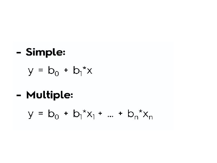
Regression • Regression is a statistical measure used in finance, investments and other disciplines that attempts to determine the strength of the relationship between one dependent variable (usually denoted by Y) and a series of other changing variables (known as independent variables). • TYPES: • Simple Linear Regression • Multi Linear Regression • Polynomial Linear Regression

Simple Linear Regression ANALYZING DATASET IV DV

Simple Linear Regression EQUATION PLOTTING SALARY (₹) y = b 0 + b 1 * x 1 SALARY = b 0 + b 1 * EXPERIENCE +10 K +1 Yr HOW much Salary will increase? +1 Yr EXPERIENCE

Simple Linear Regression Constant Coefficient y = b 0 + b 1 * x 1 Dependent variable (DV) Independent variable (IV)

Simple Linear Regression ORDINARY LEAST SQUARES • How SLR finds Best Fitting Line from our Data SALARY (₹) yi y^i Mr. ABC Modeled Observation SUM ( y - y^)2 -> min EXPERIENCE

Least Square Method • Finds the line of best fit for a dataset, providing a visual demonstration of the relationship between the data points. • The differences between the actual and estimated function values on the training examples are called residuals • The least-squares method, consists in finding ˆ f such that is minimised

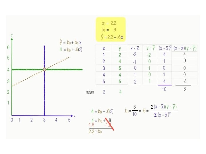
Ex: Least Square method using Univariate Regression x y x – x mean y - y mean (x – x mean)2 1 2 3 4 5 2 4 5 -2 -1 0 1 2 -2 0 1 4 1 0 1 4 (x – x mean). (y – y mean) 4 0 0 0 2

Problem Statement • Last year, five randomly selected students took a math aptitude test before they began their statistics course. The Statistics Department has three questions. • What linear regression equation best predicts statistics performance, based on math aptitude scores? • If a student made an 80 on the aptitude test, what grade would we expect her to make in statistics? • How well does the regression equation fit the data?

Student x y 1 95 85 2 85 95 3 80 70 4 70 65 5 60 70 Sum 390 385 mean 78 77 x – x mean y - y mean (x – x mean)2 (x – x mean). (y – y mean)

Libraries and Packages in Python • sklearn : – the algorithms used for data analysis and data mining tasks. • Num. Py : – It is a numeric python module which provides fast maths functions for calculations. – It is used to read data in numpy arrays and for manipulation purpose. • Pandas : – Used to read and write different files. – Data manipulation can be done easily with dataframes. • matplotlib − is 2 D plotting library for creating graphs and plots • seaborn − a data visualization library based on matplotlib

How to Find the Regression Equation • The regression equation is a linear equation of the form: ŷ = b 0 + b 1 x • First, we solve for the regression coefficient (b 1): • b 1 = Σ [ (xi - x)(yi - y) ] / Σ [ (xi - x)2] • b 1 = 470/730 • b 1 = 0. 644 • Once we know the value of the regression coefficient (b 1), we can solve for the regression slope (b 0): • b 0 = y - b 1 * x • b 0 = 77 - (0. 644)(78) • b 0 = 26. 768 • Therefore, the regression equation is: ŷ = 26. 768 + 0. 644 x.

How to Use the Regression Equation • In our example, the independent variable is the student's score on the aptitude test. • The dependent variable is the student's statistics grade. • If a student made an 80 on the aptitude test, the estimated statistics grade (ŷ) would be: • ŷ = b 0 + b 1 x • ŷ = 26. 768 + 0. 644 x = 26. 768 + 0. 644 * 80 • ŷ = 26. 768 + 51. 52 = 78. 288

How to Find the Coefficient of Determination • Whenever you use a regression equation, you should ask how well the equation fits the data. • One way to assess fit is to check the coefficient of determination, which can be computed from the following formula. • R 2 = { ( 1 / N ) * Σ [ (xi - x) * (yi - y) ] / (σx * σy ) }2 – – – – where N is the number of observations used to fit the model, Σ is the summation symbol, xi is the x value for observation i, x is the mean x value, yi is the y value for observation i, y is the mean y value, σx is the standard deviation of x, and σy is the standard deviation of y.

σx = sqrt [ Σ ( xi - x )2 / N ] σx = sqrt( 730/5 ) = sqrt(146) = 12. 083 σy = sqrt [ Σ ( yi - y )2 / N ] σy = sqrt( 630/5 ) = sqrt(126) = 11. 225 And finally, we compute the coefficient of determination (R 2): R 2 = { ( 1 / N ) * Σ [ (xi - x) * (yi - y) ] / (σx * σy ) }2 R 2 = [ ( 1/5 ) * 470 / ( 12. 083 * 11. 225 ) ]2 R 2 = ( 94 / 135. 632 )2 = ( 0. 693 )2 = 0. 48 A coefficient of determination equal to 0. 48 indicates that about 48% of the variation in statistics grades (the dependent variable) can be explained by the relationship to math aptitude scores (the independent variable). • This would be considered a good fit to the data, in the sense that it would substantially improve an educator's ability to predict student performance in statistics class. • • •

Linear regression with scikit-learn and higher dimensionality • • • from sklearn. datasets import load_boston >>> boston = load_boston() >>> boston. data. shape (506 L, 13 L) >>> boston. target. shape (506 L,

• pandas. Data. Frame(boston. data, columns=boston. feature_names)

• from sklearn. linear_model import Linear. Regression • from sklearn. model_selection import train_test_split • >>> X_train, X_test, Y_train, Y_test = train_test_split(boston. data, • boston. target, test_size=0. 1) • >>> lr = Linear. Regression(normalize=True) • >>> lr. fit(X_train, Y_train) • Linear. Regression(copy_X=True, fit_intercept=True, n_jobs=1, normalize=True)

k-fold cross-validation • The whole dataset is split into k folds using always k-1 folds for training and the remaining one to validate the model. • K iterations will be performed, using always a different validation fold • The final score can be determined as average of all values and all samples are selected for training k-1 times.

Accuracy of a regression • To check the accuracy of a regression, scikit-learn provides the internal method • score(X, y) which evaluates the model on test data: • >>> lr. score(X_test, Y_test) • 0. 77371996006718879 • Linear. Regression works with ordinary least squares, we preferred the negative mean squared error, which is a cumulative measure that must be evaluated according to the actual values (it's not relative).

Using cross_val_score() • from sklearn. model_selection import cross_val_score • >>> scores = cross_val_score(lr, boston. data, boston. target, cv=7, • scoring='neg_mean_squared_error') • array([ -11. 32601065, -10. 96365388, -32. 12770594, 33. 62294354, • -10. 55957139, -146. 42926647, -12. 98538412]) • >>> scores. mean() • -36. 859219426420601 • >>> scores. std() • 45. 704973900600457

Ridge • Ridge regression imposes an additional shrinkage penalty to the ordinary least squares loss function to limit its squared L 2 norm:

coefficient of determination or R 2. • It measures the amount of variance on the prediction which is explained by the dataset. • In other words, it is the difference between the sample and the prediction. So the R 2 is defined as follows: • For our purposes, R 2 values close to 1 mean an almost perfect regression, while values close to 0 (or negative) imply a bad model. • Using this metric is quite easy with cross-validation: • >>> cross_val_score(lr, X, Y, cv=10, scoring='r 2') • 0. 75

Regressor analytic expression • If we want to have an analytical expression of our model (a hyperplane), Linear. Regression offers two instance variables, intercept_ and coef_: • >>> print('y = ' + str(lr. intercept_) + ' ') • >>> for i, c in enumerate(lr. coef_): • print(str(c) + ' * x' + str(i))

Ridge • Ridge regression imposes an additional shrinkage penalty to the ordinary least squares loss function to limit its squared L 2 norm: • X is a matrix containing all samples as columns • w represents the weight vector. • The additional term (through the coefficient alpha—if large it implies a stronger regularization and smaller values) forces the loss function to disallow an infinite growth of w, which can be caused by multicollinearity or ill-conditioning

• • • from sklearn. datasets import load_diabetes from sklearn. linear_model import Linear. Regression, Ridge >>> diabetes = load_diabetes() >>> lr = Linear. Regression(normalize=True) >>> rg = Ridge(0. 001, normalize=True) >>> lr_scores = cross_val_score(lr, diabetes. data, diabetes. target, cv=10) >>> lr_scores. mean() 0. 46196236195833718 >>> rg_scores = cross_val_score(rg, diabetes. data, diabetes. target, cv=10) >>> rg_scores. mean() 0. 46227174692391299

• from sklearn. linear_model import Ridge. CV • >>> rg = Ridge. CV(alphas=(1. 0, 0. 1, 0. 005, 0. 0025, 0. 001, 0. 00025), • normalize=True) • >>> rg. fit(diabetes. data, diabetes. target) • >>> rg. alpha_ • 0. 005000000001

• A Lasso regressor imposes a penalty on the L 1 norm of w to determine a potentially higher number of null coefficients: • from sklearn. linear_model import Lasso • >>> ls = Lasso(alpha=0. 001, normalize=True) • >>> ls_scores = cross_val_score(ls, diabetes. data, diabetes. target, cv=10) • >>> ls_scores. mean() • 0. 46215747851504058