Part 9 Topics Statistical Inference and Regression Analysis

Part 9: Topics Statistical Inference and Regression Analysis: GB. 3302. 30 Professor William Greene Stern School of Business IOMS Department of Economics

Part 9: Topics Inference and Regression Part 9 – Linear Model Topics

Part 9: Topics 3/59 Agenda ¢ ¢ ¢ Variable Selection – Stepwise Regression Partial Regression – The Meaning of Multiple Regression Panel Data Test of Regression Stability Generalized Regression l Robust inference for OLS regression l Heteroscedasticity and weighted least squares l Autocorrelation and generalized least squares

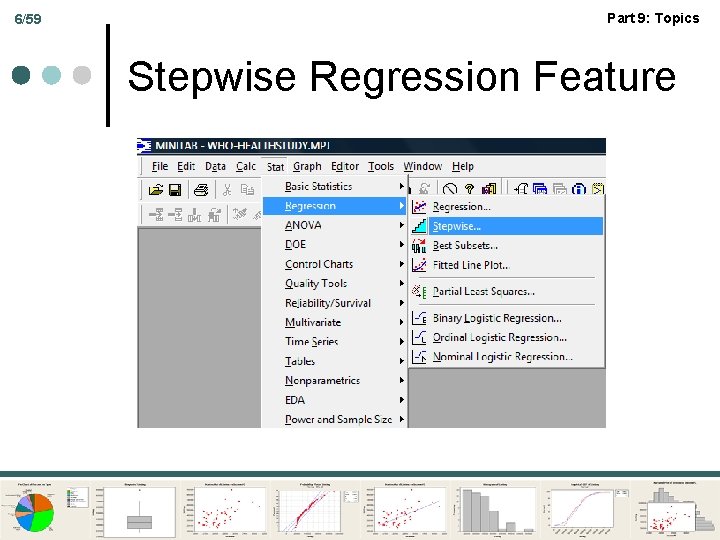
Part 9: Topics Inference and Regression Stepwise Regression

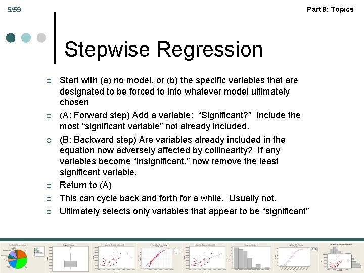
Part 9: Topics 5/59 Stepwise Regression ¢ ¢ ¢ Start with (a) no model, or (b) the specific variables that are designated to be forced to into whatever model ultimately chosen (A: Forward step) Add a variable: “Significant? ” Include the most “significant variable” not already included. (B: Backward step) Are variables already included in the equation now adversely affected by collinearity? If any variables become “insignificant, ” now remove the least significant variable. Return to (A) This can cycle back and forth for a while. Usually not. Ultimately selects only variables that appear to be “significant”

6/59 Part 9: Topics Stepwise Regression Feature

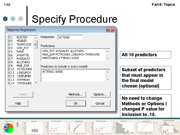
Part 9: Topics 7/59 Specify Procedure All 10 predictors Subset of predictors that must appear in the final model chosen (optional) No need to change Methods or Options I changed P value for inclusion to. 10.

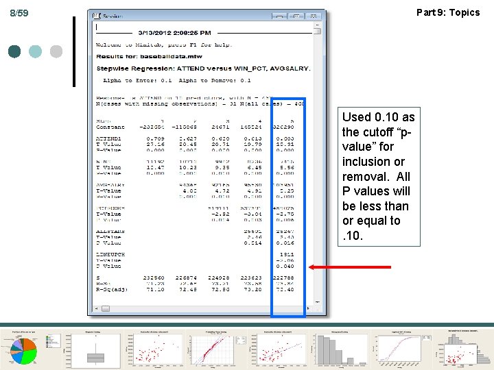
Part 9: Topics 8/59 Used 0. 10 as the cutoff “pvalue” for inclusion or removal. All P values will be less than or equal to. 10.

Part 9: Topics 9/59 Stepwise Regression ¢ What’s Right with It? l l l ¢ Automatic – push button Simple to use. Not much thinking involved. Relates in some way to connection of the variables to each other – significance – not just R 2 What’s Wrong with It? l l No reason to assume that the resulting model will make any sense Test statistics are completely invalid and cannot be used for statistical inference. (Can’t be t ratios if you know in advance they will be larger than 2. )

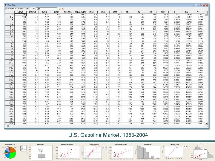
Part 9: Topics 10/59 U. S. Gasoline Market, 1953 -2004 10

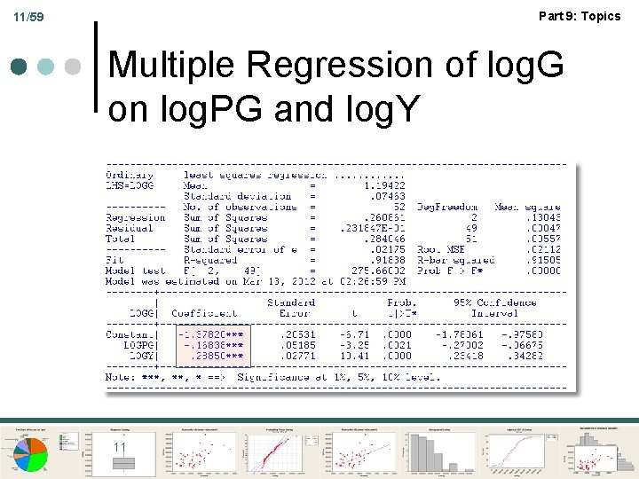
Part 9: Topics 11/59 Multiple Regression of log. G on log. PG and log. Y 11

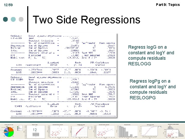
Part 9: Topics 12/59 Two Side Regressions Regress log. G on a constant and log. Y and compute residuals RESLOGG Regress log. Pg on a constant and log. Y and compute residuals RESLOGPG 12

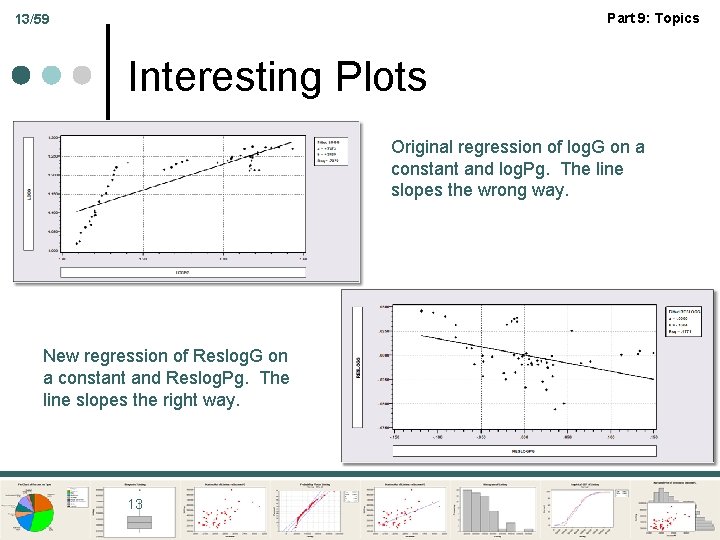
Part 9: Topics 13/59 Interesting Plots Original regression of log. G on a constant and log. Pg. The line slopes the wrong way. New regression of Reslog. G on a constant and Reslog. Pg. The line slopes the right way. 13

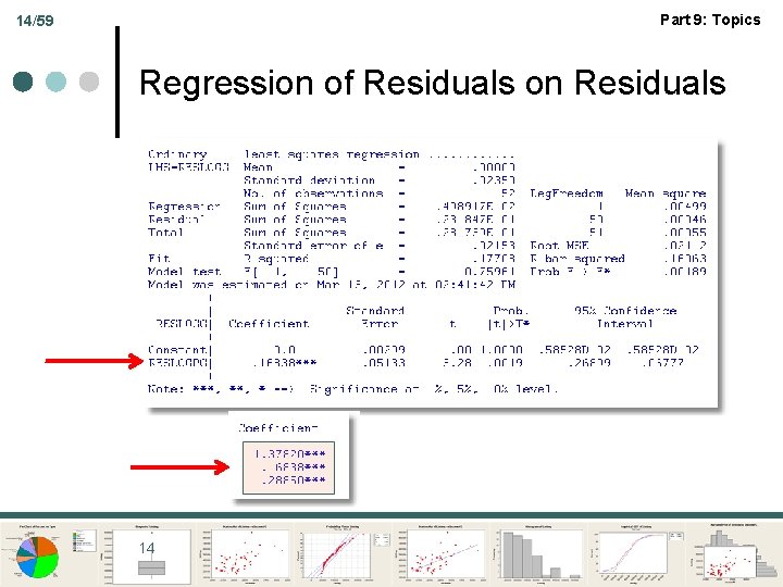
Part 9: Topics 14/59 Regression of Residuals on Residuals 14

Part 9: Topics 15/59 Frisch-Waugh Result “We get the same result whether we (1) detrend the other variables by using the residuals from a regression of them on a constant and a time trend and use the detrended data in the regression or (2) just include a constant and a time trend in the regression and not detrend the data” “Detrend the data” means compute the residuals from the regressions of the variables on a constant and a time trend.

Part 9: Topics 16/59 Understanding Multiple Regresion ¢ ¢ ¢ In a multiple regression, the coefficient on an x is interpreted to give the effect of change in x on change in y holding everything else constant. That is, “net of the effect of everything else. ” How can y=a+b 1 Educ+b 2 Age+e? Each year of education means aging by 1 year. How is it possible to hold age constant and increase education by 1 year? 16

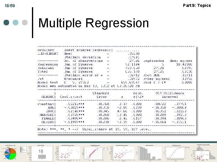
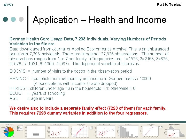
Part 9: Topics 17/59 Application – Health and Income German Health Care Usage Data, 7, 293 Individuals, Varying Numbers of Periods Variables in the file are Data downloaded from Journal of Applied Econometrics Archive. This is an unbalanced panel with 7, 293 individuals. There altogether 27, 326 observations. The number of observations ranges from 1 to 7 per family. (Frequencies are: 1=1525, 2=2158, 3=825, 4=926, 5=1051, 6=1000, 7=987). The dependent variable of interest is DOCVIS = number of visits to the doctor in the observation period HHNINC = household nominal monthly net income in German marks / 10000. (4 observations with income=0 were dropped) HHKIDS = children under age 16 in the household = 1; otherwise = 0 EDUC = years of schooling AGE = age in years

Part 9: Topics 18/59 Multiple Regression 18

Part 9: Topics Inference and Regression Panel Data

Part 9: Topics Inference and Regression A Case Study

Part 9: Topics 21/59 Mega Deals for Stars A Capital Budgeting Computation ¢ Costs and Benefits ¢ Certainty: Costs l Uncertainty: Benefits l ¢ Long Term: Need for discounting

Part 9: Topics 22/59 Baseball Story A Huge Sports Contract ¢ ¢ Alex Rodriguez hired by the Texas Rangers for something like $25 million per year in 2000. Costs – the salary plus and minus some fine tuning of the numbers Benefits – more fans in the stands. How to determine if the benefits exceed the costs? Use a regression model.

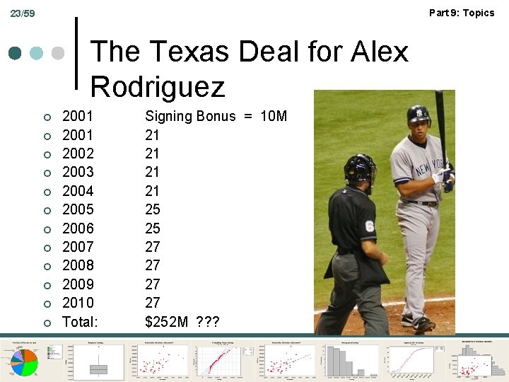
Part 9: Topics 23/59 The Texas Deal for Alex Rodriguez ¢ ¢ ¢ 2001 2002 2003 2004 2005 2006 2007 2008 2009 2010 Total: Signing Bonus = 10 M 21 21 25 25 27 27 $252 M ? ? ?

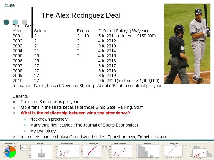
Part 9: Topics 24/59 The Alex Rodriguez Deal Direct Costs Year Salary Bonus 2001 21 2 + 10 2002 21 2 2003 21 2 2004 21 2 2005 25 2 2006 25 2007 27 2008 27 2009 27 2010 27 Insurance, Taxes, Loss of Revenue Sharing: Deferred Salary (3%/year) 5 to 2011 (+Interest $150, 000) 4 to 2012 … 3 to 2013 4 to 2014 4 to 2015 4 to 2016 3 to 2017 3 to 2018 3 to 2019 5 to 2020 (+Interest > 1, 000) About 50% of the contract per year Benefits ¢ Projected 8 more wins per year ¢ More fans in the seats because of those wins: Gate, Parking, Stuff ¢ What is the relationship between wins and attendance? l Not known precisely l Many empirical studies (The Journal of Sports Economics) l My own study ¢ Increased chance at playoffs and world series: Sponshorships, Franchise Value

Part 9: Topics 25/59 Costs ¢ ¢ ¢ Insurance: About 10% of the contract per year (Taxes: About 40% of the contract) Some additional costs in revenue sharing revenues from the league (anticipated, about 17. 5% of marginal benefits – uncertain) Interest on deferred salary - $150, 000 in first year, well over $1, 000 in 2010. (Reduction) $3 M it would cost to have a different shortstop. (Nomar Garciaparra)

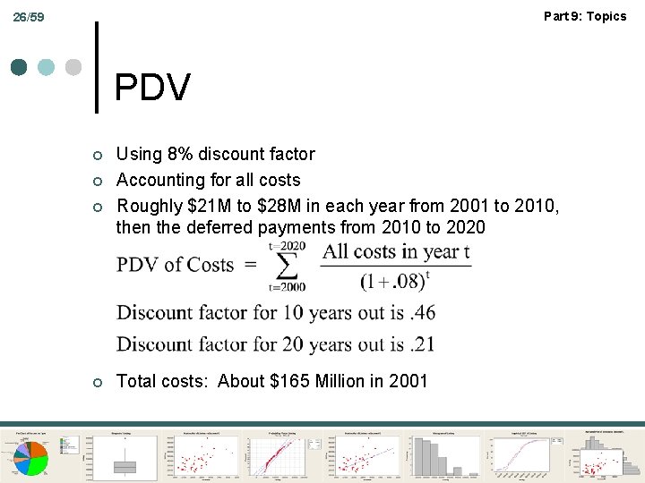
Part 9: Topics 26/59 PDV ¢ ¢ Using 8% discount factor Accounting for all costs Roughly $21 M to $28 M in each year from 2001 to 2010, then the deferred payments from 2010 to 2020 Total costs: About $165 Million in 2001

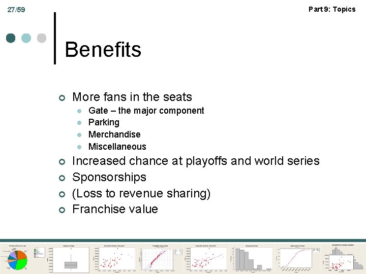
Part 9: Topics 27/59 Benefits ¢ More fans in the seats l l ¢ ¢ Gate – the major component Parking Merchandise Miscellaneous Increased chance at playoffs and world series Sponsorships (Loss to revenue sharing) Franchise value

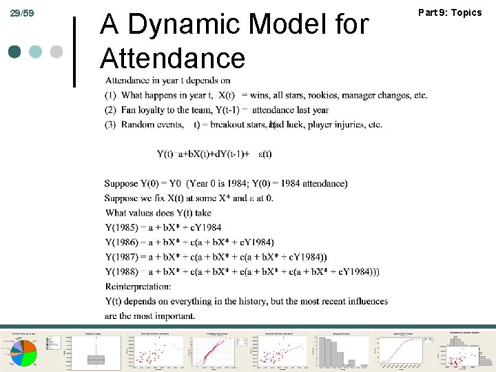
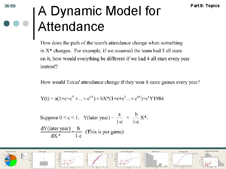
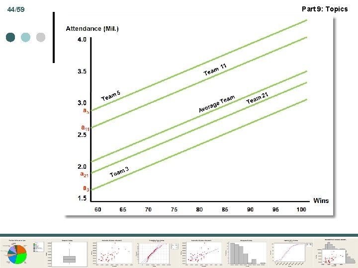
Part 9: Topics 28/59 How Many New Fans? Projected 8 more wins per year. ¢ What is the relationship between wins and attendance? ¢ Not known precisely l Many empirical studies (The Journal of Sports Economics) l My own study… l

29/59 A Dynamic Model for Attendance Part 9: Topics

30/59 A Dynamic Model for Attendance Part 9: Topics

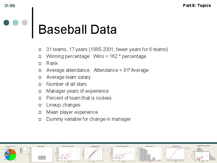
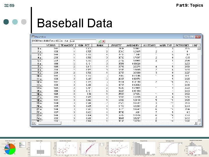
Part 9: Topics 31/59 Baseball Data ¢ ¢ ¢ 31 teams, 17 years (1985 -2001; fewer years for 6 teams) Winning percentage: Wins = 162 * percentage Rank Average attendance. Attendance = 81*Average team salary Number of all stars Manager years of experience Percent of team that is rookies Lineup changes Mean player experience Dummy variable for change in manager

Part 9: Topics 32/59 Baseball Data

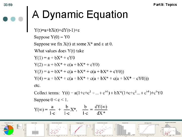
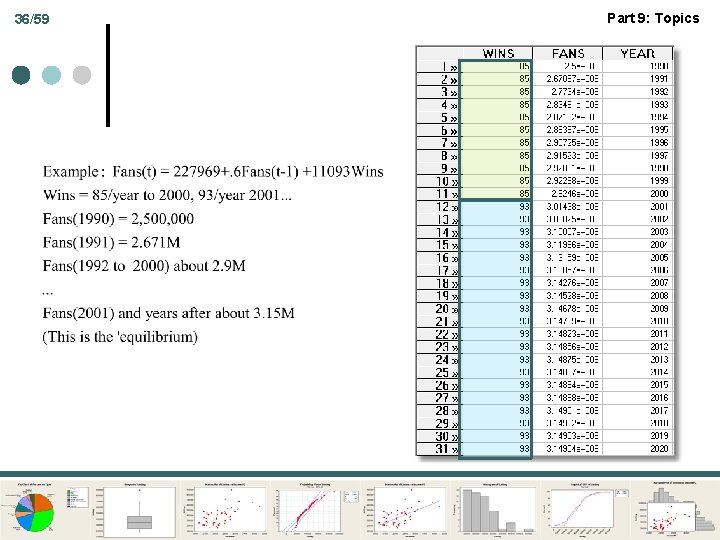
Part 9: Topics 33/59 A Dynamic Equation

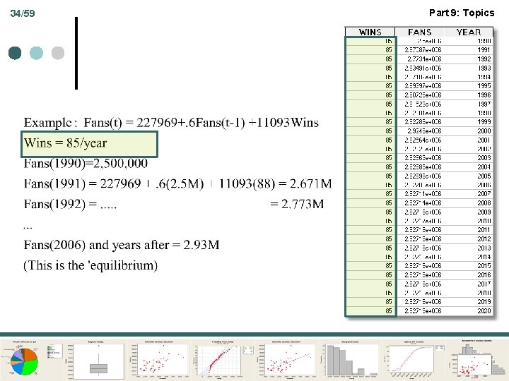
34/59 Part 9: Topics

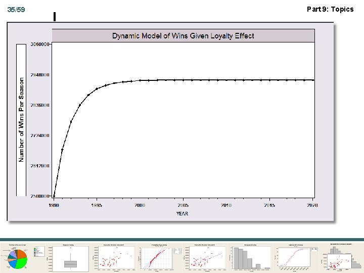
35/59 Part 9: Topics

36/59 Part 9: Topics

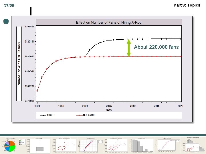
37/59 Part 9: Topics About 220, 000 fans

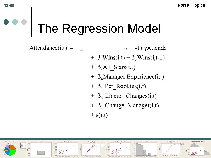
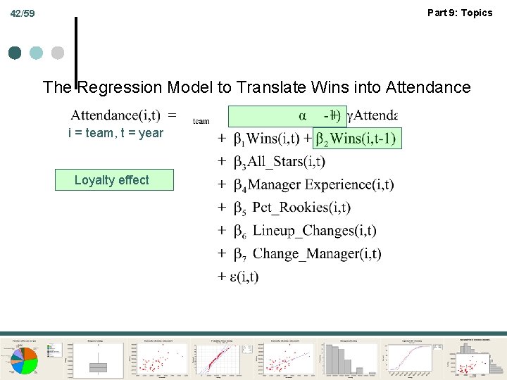
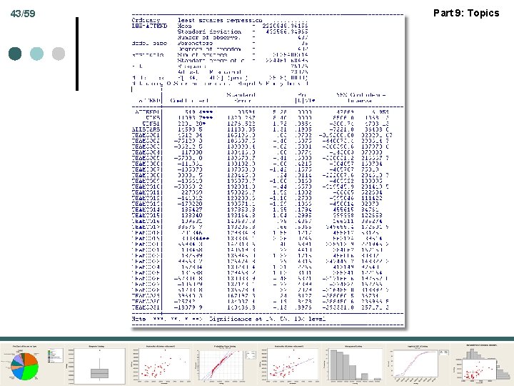
Part 9: Topics 38/59 The Regression Model

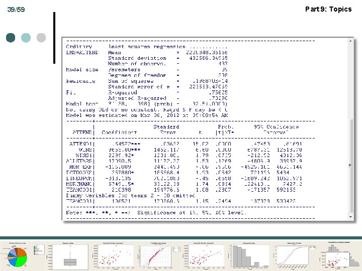
39/59 Part 9: Topics

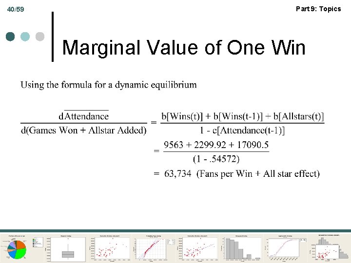
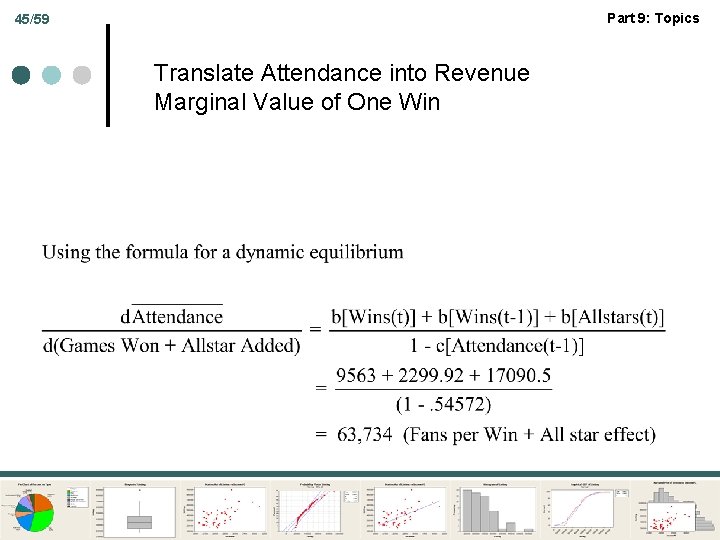
40/59 Part 9: Topics Marginal Value of One Win

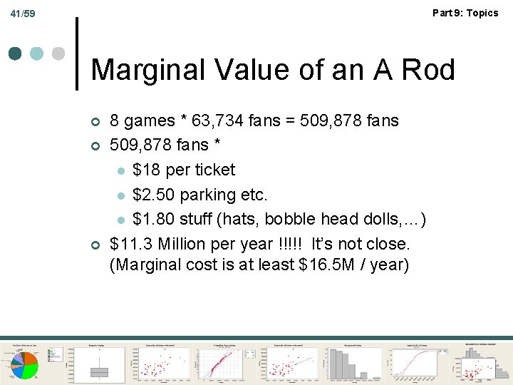
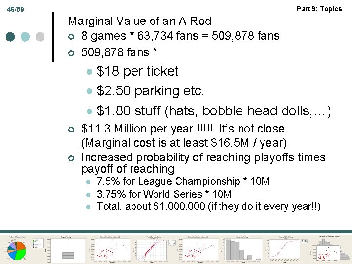
Part 9: Topics 41/59 Marginal Value of an A Rod ¢ ¢ ¢ 8 games * 63, 734 fans = 509, 878 fans * l $18 per ticket l $2. 50 parking etc. l $1. 80 stuff (hats, bobble head dolls, …) $11. 3 Million per year !!!!! It’s not close. (Marginal cost is at least $16. 5 M / year)

Part 9: Topics 42/59 The Regression Model to Translate Wins into Attendance i = team, t = year Loyalty effect

43/59 Part 9: Topics

44/59 Part 9: Topics

Part 9: Topics 45/59 Translate Attendance into Revenue Marginal Value of One Win

Part 9: Topics 46/59 Marginal Value of an A Rod ¢ 8 games * 63, 734 fans = 509, 878 fans ¢ 509, 878 fans * $18 per ticket l $2. 50 parking etc. l $1. 80 stuff (hats, bobble head dolls, …) l ¢ ¢ $11. 3 Million per year !!!!! It’s not close. (Marginal cost is at least $16. 5 M / year) Increased probability of reaching playoffs times payoff of reaching l l l 7. 5% for League Championship * 10 M 3. 75% for World Series * 10 M Total, about $1, 000 (if they do it every year!!)

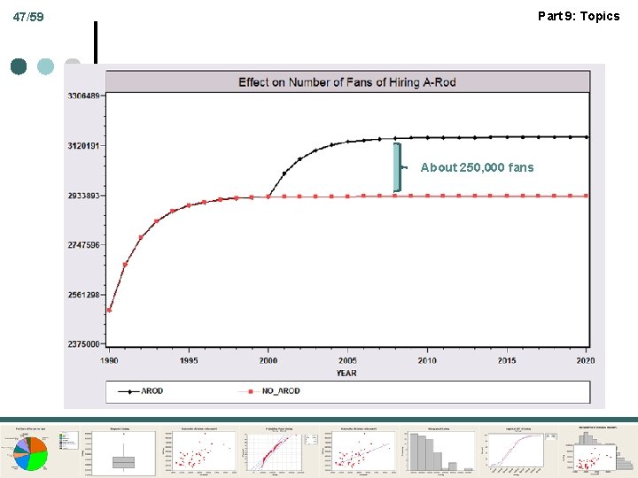
Part 9: Topics 47/59 About 250, 000 fans

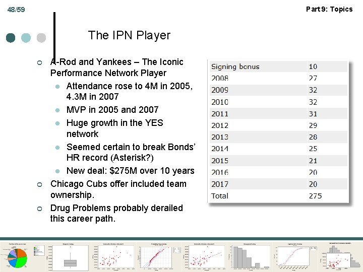
Part 9: Topics 48/59 The IPN Player ¢ ¢ ¢ A-Rod and Yankees – The Iconic Performance Network Player l Attendance rose to 4 M in 2005, 4. 3 M in 2007 l MVP in 2005 and 2007 l Huge growth in the YES network l Seemed certain to break Bonds’ HR record (Asterisk? ) l New deal: $275 M over 10 years Chicago Cubs offer included team ownership. Drug Problems probably derailed this career path.

Part 9: Topics 49/59 Application – Health and Income German Health Care Usage Data, 7, 293 Individuals, Varying Numbers of Periods Variables in the file are Data downloaded from Journal of Applied Econometrics Archive. This is an unbalanced panel with 7, 293 individuals. There altogether 27, 326 observations. The number of observations ranges from 1 to 7 per family. (Frequencies are: 1=1525, 2=2158, 3=825, 4=926, 5=1051, 6=1000, 7=987). The dependent variable of interest is DOCVIS = number of visits to the doctor in the observation period HHNINC = household nominal monthly net income in German marks / 10000. (4 observations with income=0 were dropped) HHKIDS = children under age 16 in the household = 1; otherwise = 0 EDUC = years of schooling AGE = age in years We desire also to include a separate family effect (7293 of them) for each family. This requires 7293 dummy variables in addition to the four regressors.

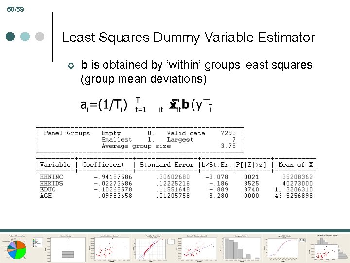
50/59 Least Squares Dummy Variable Estimator ¢ b is obtained by ‘within’ groups least squares (group mean deviations)

Part 9: Topics Inference and Regression Chow Test

Part 9: Topics 52/59 Equal Regressions Setting: Two groups of observations (men/women, countries, two different periods, firms, etc. ) ¢ Regression Model: y = α+β 1 x 1+β 2 x 2 + … + ε ¢ Hypothesis: The same model applies to both groups ¢ Rejection region: Large values of F ¢

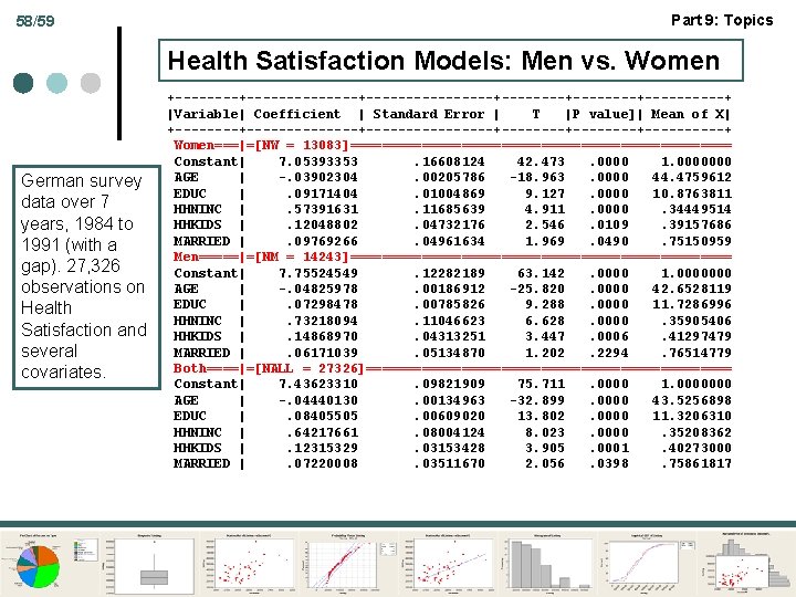
Part 9: Topics 53/59 Application ¢ Health satisfaction depends on many factors: l l ¢ ¢ ¢ Age, Income, Children, Education, Marital Status Do these factors figure differently in a model for women compared to men? Investigation: Multiple regression Hypothesis: The regressions are the same. Rejection Region: Estimated regressions that are very different.

Part 9: Topics 54/59 Test of Structural Stability Two groups, cleverly labeled Group 1 and Group 2. Regression model applies to the two groups: y j = X j j + j Null hypothesis: 1 = 2 Test using an F statistic. 54

Part 9: Topics 55/59 Testing Strategy: Setup ¢ Fit separate regressions for the two groups. l l ¢ Pooled regression l l ¢ Separate coefficient vectors b 1 and b 2 Each coefficient vector is bj = (Xj’Xj)-1 Xj’yj Sums of squares e 1’e 1 = (y 1 - X 1 b 1)’(y 1 - X 1 b 1) and e 2’e 2 = (y 2 – X 2 b 2)’(y 2 – X 2 b 2) Total separate sum of squares = SS 12 = e 1’e 1 + e 2’e 2 b = (X 1’X 1 + X 2’X 2)-1 ( X 1’y 1 + X 2’y 2) Pooled sum of squares SSpooled = e 1’e 1 = (y 1 - X 1 b)’(y 1 - X 1 b) + (y 2 – X 2 b)’(y 2 – X 2 b) SSpooled must be > SS 12

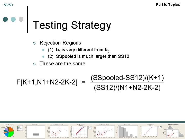
Part 9: Topics 56/59 Testing Strategy ¢ Rejection Regions l l ¢ (1) b 1 is very different from b 2 (2) SSpooled is much larger than SS 12 These are the same.

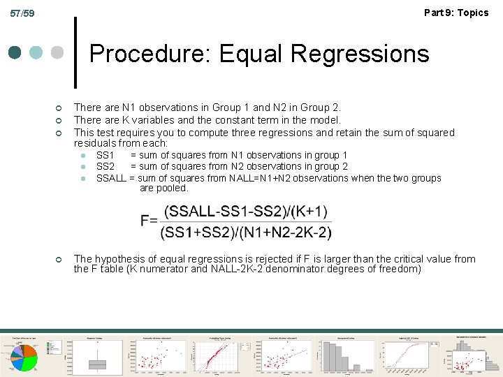
Part 9: Topics 57/59 Procedure: Equal Regressions ¢ ¢ ¢ There are N 1 observations in Group 1 and N 2 in Group 2. There are K variables and the constant term in the model. This test requires you to compute three regressions and retain the sum of squared residuals from each: l l l ¢ SS 1 = sum of squares from N 1 observations in group 1 SS 2 = sum of squares from N 2 observations in group 2 SSALL = sum of squares from NALL=N 1+N 2 observations when the two groups are pooled. The hypothesis of equal regressions is rejected if F is larger than the critical value from the F table (K numerator and NALL-2 K-2 denominator degrees of freedom)

58/59 Part 9: Topics Health Satisfaction Models: Men vs. Women German survey data over 7 years, 1984 to 1991 (with a gap). 27, 326 observations on Health Satisfaction and several covariates. +--------------+--------+--------+-----+ |Variable| Coefficient | Standard Error | T |P value]| Mean of X| +--------------+--------+--------+-----+ Women===|=[NW = 13083]======================== Constant| 7. 05393353. 16608124 42. 473. 0000 1. 0000000 AGE | -. 03902304. 00205786 -18. 963. 0000 44. 4759612 EDUC |. 09171404. 01004869 9. 127. 0000 10. 8763811 HHNINC |. 57391631. 11685639 4. 911. 0000. 34449514 HHKIDS |. 12048802. 04732176 2. 546. 0109. 39157686 MARRIED |. 09769266. 04961634 1. 969. 0490. 75150959 Men=====|=[NM = 14243]======================== Constant| 7. 75524549. 12282189 63. 142. 0000 1. 0000000 AGE | -. 04825978. 00186912 -25. 820. 0000 42. 6528119 EDUC |. 07298478. 00785826 9. 288. 0000 11. 7286996 HHNINC |. 73218094. 11046623 6. 628. 0000. 35905406 HHKIDS |. 14868970. 04313251 3. 447. 0006. 41297479 MARRIED |. 06171039. 05134870 1. 202. 2294. 76514779 Both====|=[NALL = 27326]======================= Constant| 7. 43623310. 09821909 75. 711. 0000000 AGE | -. 04440130. 00134963 -32. 899. 0000 43. 5256898 EDUC |. 08405505. 00609020 13. 802. 0000 11. 3206310 HHNINC |. 64217661. 08004124 8. 023. 0000. 35208362 HHKIDS |. 12315329. 03153428 3. 905. 0001. 40273000 MARRIED |. 07220008. 03511670 2. 056. 0398. 75861817

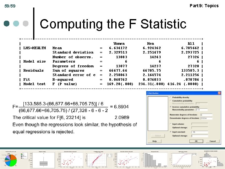
Part 9: Topics 59/59 Computing the F Statistic +----------------------------------------+ | Women Men All | | LHS=HEALTH Mean = 6. 634172 6. 924362 6. 785662 | | Standard deviation = 2. 329513 2. 251479 2. 293725 | | Number of observs. = 13083 14243 27326 | | Model size Parameters = 6 6 6 | | Degrees of freedom = 13077 14237 27320 | | Residuals Sum of squares = 66677. 66 66705. 75 133585. 3 | | Standard error of e = 2. 258063 2. 164574 2. 211256 | | Fit R-squared = 0. 060762 0. 076033. 070786 | | Model test F (P value) = 169. 20(. 000) 234. 31(. 000) 416. 24 (. 0000) | +----------------------------------------+