Part 8 Regression Model Statistical Inference and Regression

Part 8: Regression Model Statistical Inference and Regression Analysis: GB. 3302. 30 Professor William Greene Stern School of Business IOMS Department of Economics

Part 8: Regression Model Inference and Regression Perfect Collinearity

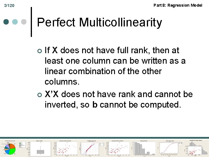
Part 8: Regression Model 3/120 Perfect Multicollinearity If X does not have full rank, then at least one column can be written as a linear combination of the other columns. ¢ X’X does not have rank and cannot be inverted, so b cannot be computed. ¢

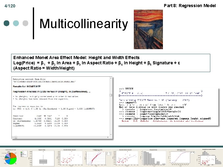
Part 8: Regression Model 4/120 Multicollinearity Enhanced Monet Area Effect Model: Height and Width Effects Log(Price) = β 1 + β 2 ln Area + β 3 ln Aspect Ratio + β 4 ln Height + β 5 Signature + ε (Aspect Ratio = Width/Height)

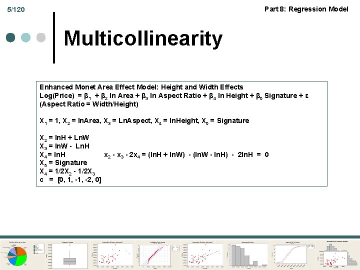
Part 8: Regression Model 5/120 Multicollinearity Enhanced Monet Area Effect Model: Height and Width Effects Log(Price) = β 1 + β 2 ln Area + β 3 ln Aspect Ratio + β 4 ln Height + β 5 Signature + ε (Aspect Ratio = Width/Height) X 1 = 1, X 2 = ln. Area, X 3 = Ln. Aspect, X 4 = ln. Height, X 5 = Signature X 2 = ln. H + Ln. W X 3 = ln. W - Ln. H X 4 = ln. H x 2 - x 3 - 2 x 4 = (ln. H + ln. W) - (ln. W - ln. H) - 2 ln. H = 0 X 5 = Signature X 4 = 1/2 X 2 - 1/2 X 3 c = [0, 1, -2, 0]

Part 8: Regression Model Inference and Regression Least Squares Fit

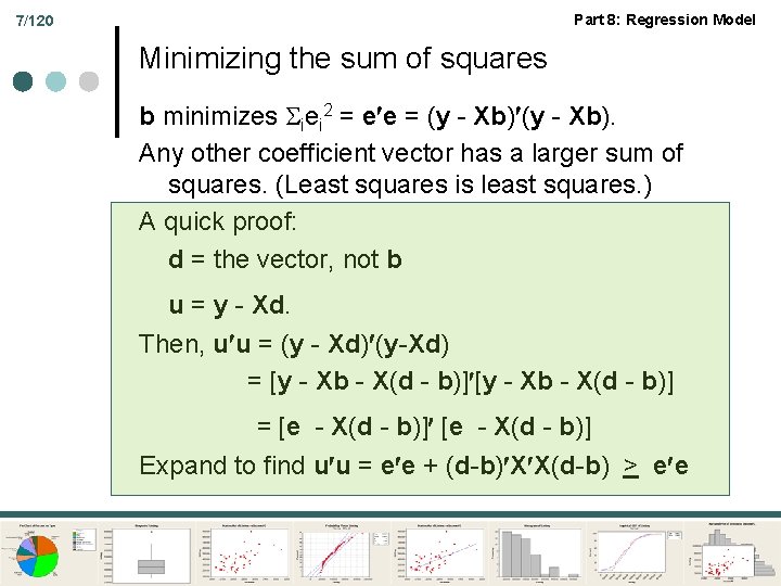
Part 8: Regression Model 7/120 Minimizing the sum of squares b minimizes iei 2 = e e = (y - Xb). Any other coefficient vector has a larger sum of squares. (Least squares is least squares. ) A quick proof: d = the vector, not b u = y - Xd. Then, u u = (y - Xd) (y-Xd) = [y - Xb - X(d - b)] = [e - X(d - b)] Expand to find u u = e e + (d-b) X X(d-b) > e e

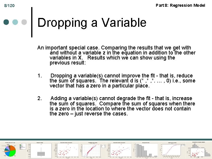
Part 8: Regression Model 8/120 Dropping a Variable An important special case. Comparing the results that we get with and without a variable z in the equation in addition to the other variables in X. Results which we can show using the previous result: 1. Dropping a variable(s) cannot improve the fit - that is, reduce the sum of squares. The relevant d is (* , *. … , 0) i. e. , some vector that has a zero in a particular place. 2. Adding a variable(s) cannot degrade the fit - that is, increase the sum of squares. Compare the sum of squares when there is a zero in the location to where the vector does not contain the zero – just reverse the cases.

9/120 Part 8: Regression Model The Fit of the Regression “Variation: ” In the context of the “model” we speak of variation of a variable as movement of the variable, usually associated with (not necessarily caused by) movement of another variable.

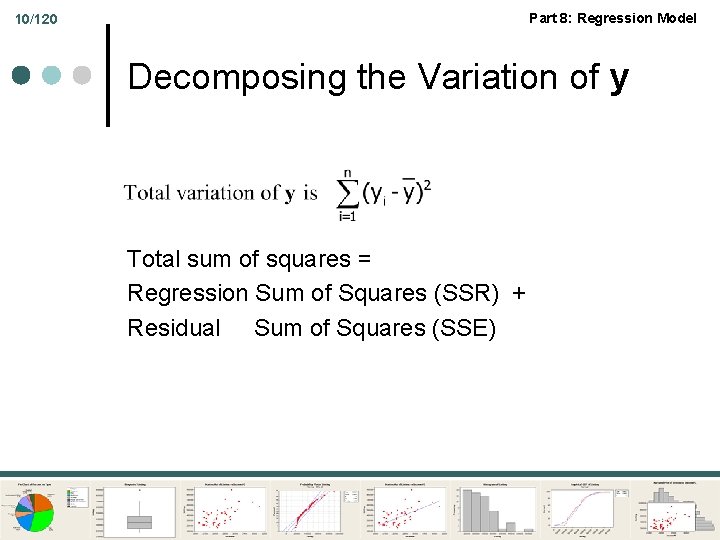
Part 8: Regression Model 10/120 Decomposing the Variation of y Total sum of squares = Regression Sum of Squares (SSR) + Residual Sum of Squares (SSE)

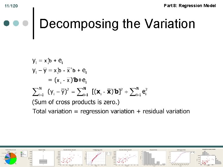
11/120 Part 8: Regression Model Decomposing the Variation

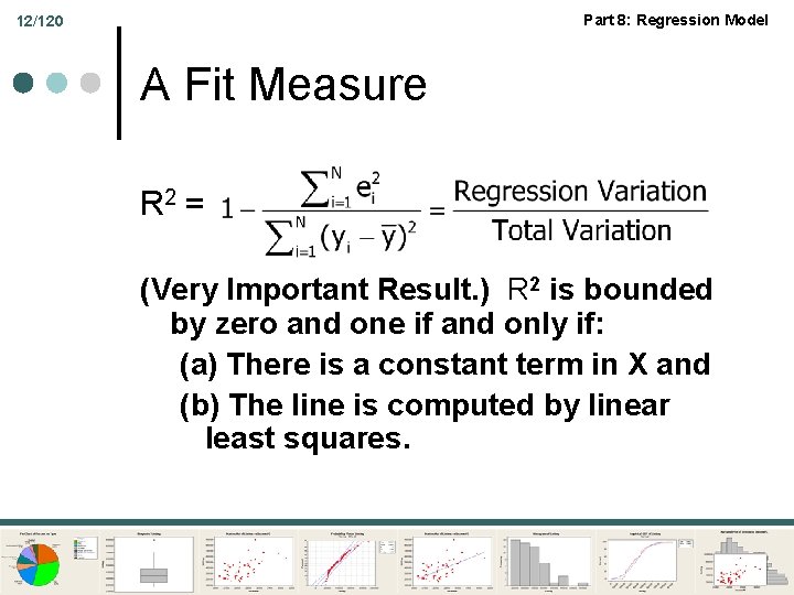
Part 8: Regression Model 12/120 A Fit Measure R 2 = (Very Important Result. ) R 2 is bounded by zero and one if and only if: (a) There is a constant term in X and (b) The line is computed by linear least squares.

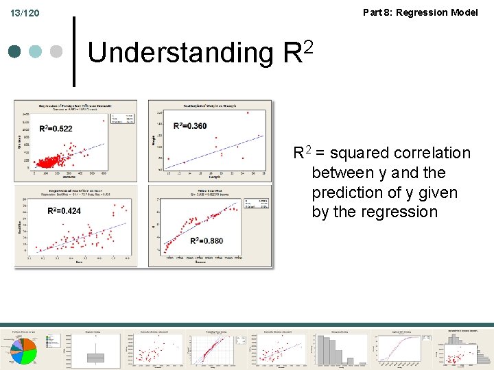
Part 8: Regression Model 13/120 Understanding R 2 = squared correlation between y and the prediction of y given by the regression

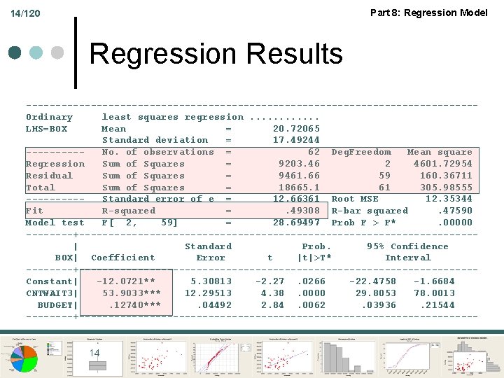
Part 8: Regression Model 14/120 Regression Results --------------------------------------Ordinary least squares regression. . . LHS=BOX Mean = 20. 72065 Standard deviation = 17. 49244 -----No. of observations = 62 Deg. Freedom Mean square Regression Sum of Squares = 9203. 46 2 4601. 72954 Residual Sum of Squares = 9461. 66 59 160. 36711 Total Sum of Squares = 18665. 1 61 305. 98555 -----Standard error of e = 12. 66361 Root MSE 12. 35344 Fit R-squared =. 49308 R-bar squared. 47590 Model test F[ 2, 59] = 28. 69497 Prob F > F*. 00000 ----+----------------------------------| Standard Prob. 95% Confidence BOX| Coefficient Error t |t|>T* Interval ----+----------------------------------Constant| -12. 0721** 5. 30813 -2. 27. 0266 -22. 4758 -1. 6684 CNTWAIT 3| 53. 9033*** 12. 29513 4. 38. 0000 29. 8053 78. 0013 BUDGET|. 12740***. 04492 2. 84. 0062. 03936. 21544 ----+---------------------------------- 14

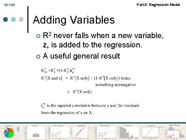
Part 8: Regression Model 15/120 Adding Variables R 2 never falls when a new variable, z, is added to the regression. ¢ A useful general result ¢

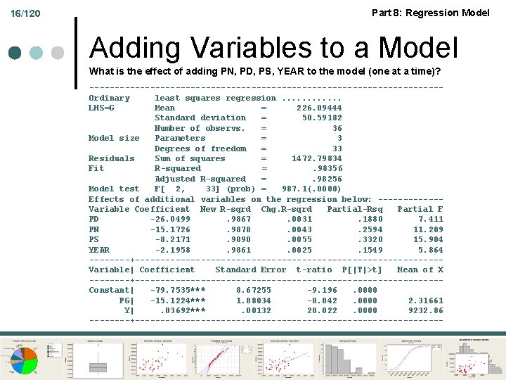
16/120 Part 8: Regression Model Adding Variables to a Model What is the effect of adding PN, PD, PS, YEAR to the model (one at a time)? -----------------------------------Ordinary least squares regression. . . LHS=G Mean = 226. 09444 Standard deviation = 50. 59182 Number of observs. = 36 Model size Parameters = 3 Degrees of freedom = 33 Residuals Sum of squares = 1472. 79834 Fit R-squared =. 98356 Adjusted R-squared =. 98256 Model test F[ 2, 33] (prob) = 987. 1(. 0000) Effects of additional variables on the regression below: ------Variable Coefficient New R-sqrd Chg. R-sqrd Partial-Rsq Partial F PD -26. 0499. 9867. 0031. 1880 7. 411 PN -15. 1726. 9878. 0043. 2594 11. 209 PS -8. 2171. 9890. 0055. 3320 15. 904 YEAR -2. 1958. 9861. 0025. 1549 5. 864 ----+------------------------------Variable| Coefficient Standard Error t-ratio P[|T|>t] Mean of X ----+------------------------------Constant| -79. 7535*** 8. 67255 -9. 196. 0000 PG| -15. 1224*** 1. 88034 -8. 042. 0000 2. 31661 Y|. 03692***. 00132 28. 022. 0000 9232. 86 ----+-------------------------------

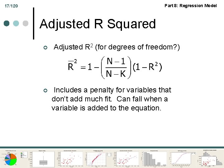
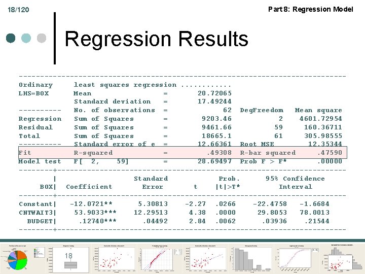
Part 8: Regression Model 17/120 Adjusted R Squared ¢ ¢ Adjusted R 2 (for degrees of freedom? ) Includes a penalty for variables that don’t add much fit. Can fall when a variable is added to the equation.

Part 8: Regression Model 18/120 Regression Results --------------------------------------Ordinary least squares regression. . . LHS=BOX Mean = 20. 72065 Standard deviation = 17. 49244 -----No. of observations = 62 Deg. Freedom Mean square Regression Sum of Squares = 9203. 46 2 4601. 72954 Residual Sum of Squares = 9461. 66 59 160. 36711 Total Sum of Squares = 18665. 1 61 305. 98555 -----Standard error of e = 12. 66361 Root MSE 12. 35344 Fit R-squared =. 49308 R-bar squared. 47590 Model test F[ 2, 59] = 28. 69497 Prob F > F*. 00000 ----+----------------------------------| Standard Prob. 95% Confidence BOX| Coefficient Error t |t|>T* Interval ----+----------------------------------Constant| -12. 0721** 5. 30813 -2. 27. 0266 -22. 4758 -1. 6684 CNTWAIT 3| 53. 9033*** 12. 29513 4. 38. 0000 29. 8053 78. 0013 BUDGET|. 12740***. 04492 2. 84. 0062. 03936. 21544 ----+---------------------------------- 18

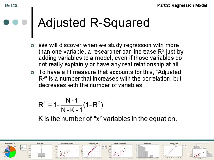
Part 8: Regression Model 19/120 Adjusted R-Squared ¢ ¢ We will discover when we study regression with more than one variable, a researcher can increase R 2 just by adding variables to a model, even if those variables do not really explain y or have any real relationship at all. To have a fit measure that accounts for this, “Adjusted R 2” is a number that increases with the correlation, but decreases with the number of variables.

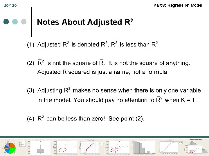
Part 8: Regression Model 20/120 Notes About Adjusted R 2

Part 8: Regression Model Inference and Regression Transformed Data

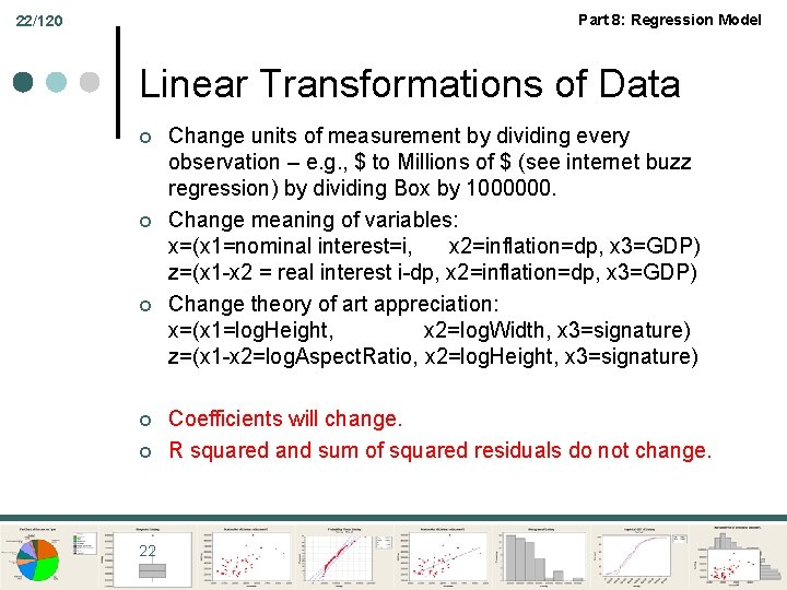
Part 8: Regression Model 22/120 Linear Transformations of Data ¢ ¢ ¢ 22 Change units of measurement by dividing every observation – e. g. , $ to Millions of $ (see internet buzz regression) by dividing Box by 1000000. Change meaning of variables: x=(x 1=nominal interest=i, x 2=inflation=dp, x 3=GDP) z=(x 1 -x 2 = real interest i-dp, x 2=inflation=dp, x 3=GDP) Change theory of art appreciation: x=(x 1=log. Height, x 2=log. Width, x 3=signature) z=(x 1 -x 2=log. Aspect. Ratio, x 2=log. Height, x 3=signature) Coefficients will change. R squared and sum of squared residuals do not change.

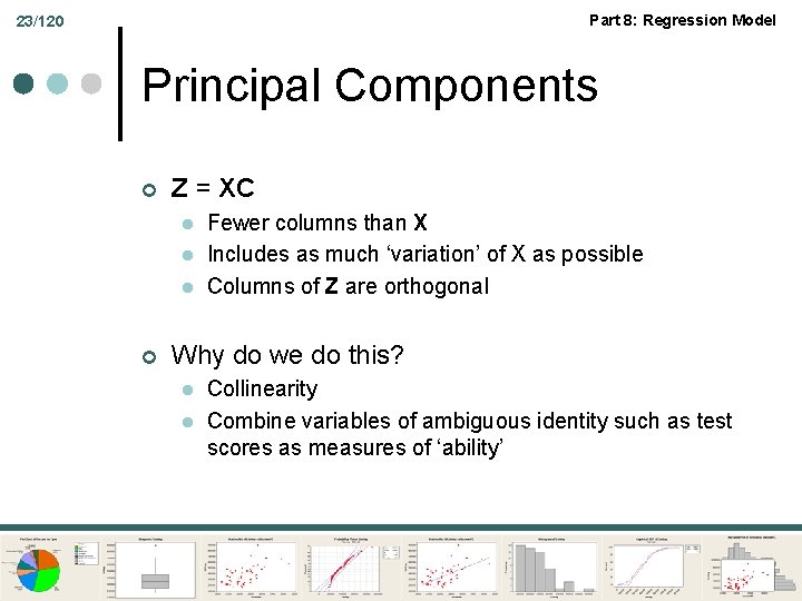
Part 8: Regression Model 23/120 Principal Components ¢ Z = XC l l l ¢ Fewer columns than X Includes as much ‘variation’ of X as possible Columns of Z are orthogonal Why do we do this? l l Collinearity Combine variables of ambiguous identity such as test scores as measures of ‘ability’

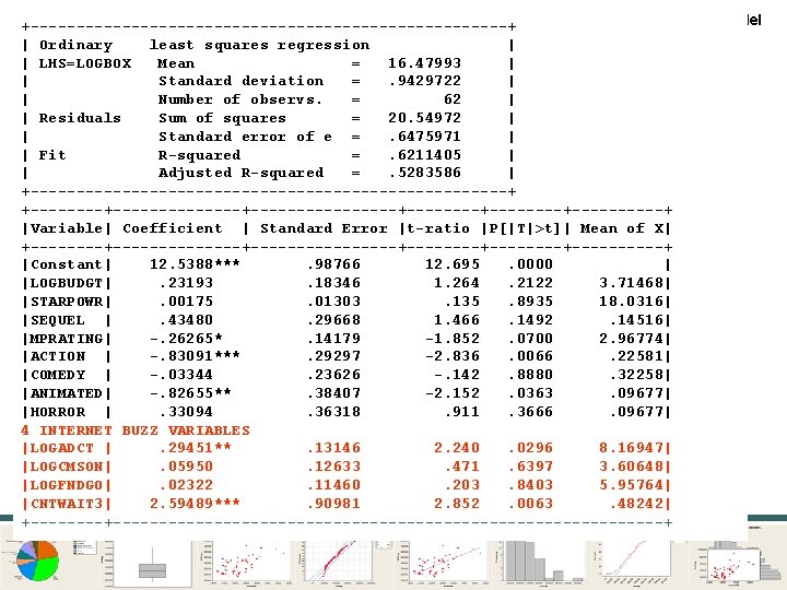
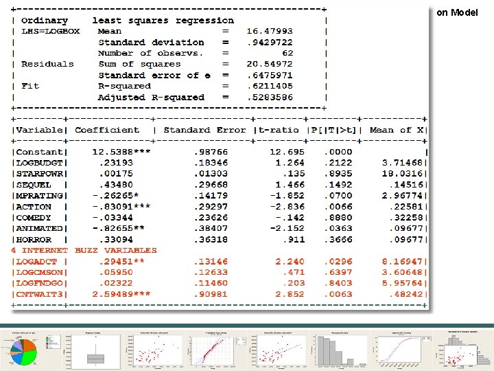
Part 8: Regression Model 24/120 +--------------------------+ | Ordinary least squares regression | | LHS=LOGBOX Mean = 16. 47993 | | Standard deviation =. 9429722 | | Number of observs. = 62 | | Residuals Sum of squares = 20. 54972 | | Standard error of e =. 6475971 | | Fit R-squared =. 6211405 | | Adjusted R-squared =. 5283586 | +--------------------------+ +--------------+--------+--------+-----+ |Variable| Coefficient | Standard Error |t-ratio |P[|T|>t]| Mean of X| +--------------+--------+--------+-----+ |Constant| 12. 5388***. 98766 12. 695. 0000 | |LOGBUDGT|. 23193. 18346 1. 264. 2122 3. 71468| |STARPOWR|. 00175. 01303. 135. 8935 18. 0316| |SEQUEL |. 43480. 29668 1. 466. 1492. 14516| |MPRATING| -. 26265*. 14179 -1. 852. 0700 2. 96774| |ACTION | -. 83091***. 29297 -2. 836. 0066. 22581| |COMEDY | -. 03344. 23626 -. 142. 8880. 32258| |ANIMATED| -. 82655**. 38407 -2. 152. 0363. 09677| |HORROR |. 33094. 36318. 911. 3666. 09677| 4 INTERNET BUZZ VARIABLES |LOGADCT |. 29451**. 13146 2. 240. 0296 8. 16947| |LOGCMSON|. 05950. 12633. 471. 6397 3. 60648| |LOGFNDGO|. 02322. 11460. 203. 8403 5. 95764| |CNTWAIT 3| 2. 59489***. 90981 2. 852. 0063. 48242| +----------------------------------+

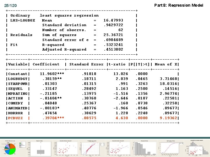
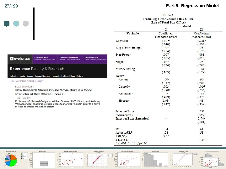
Part 8: Regression Model 25/120 +--------------------------+ | Ordinary least squares regression | | LHS=LOGBOX Mean = 16. 47993 | | Standard deviation =. 9429722 | | Number of observs. = 62 | | Residuals Sum of squares = 25. 36721 | | Standard error of e =. 6984489 | | Fit R-squared =. 5323241 | | Adjusted R-squared =. 4513802 | +--------------------------+ +--------------+--------+--------+-----+ |Variable| Coefficient | Standard Error |t-ratio |P[|T|>t]| Mean of X| +--------------+--------+--------+-----+ |Constant| 11. 9602***. 91818 13. 026. 0000 | |LOGBUDGT|. 38159**. 18711 2. 039. 0465 3. 71468| |STARPOWR|. 01303. 01315. 991. 3263 18. 0316| |SEQUEL |. 33147. 28492 1. 163. 2500. 14516| |MPRATING| -. 21185. 13975 -1. 516. 1356 2. 96774| |ACTION | -. 81404**. 30760 -2. 646. 0107. 22581| |COMEDY |. 04048. 25367. 160. 8738. 32258| |ANIMATED| -. 80183*. 40776 -1. 966. 0546. 09677| |HORROR |. 47454. 38629 1. 228. 2248. 09677| |PCBUZZ |. 39704***. 08575 4. 630. 0000 9. 19362| +----------------------------------+

26/120 Part 8: Regression Model

27/120 Part 8: Regression Model

Part 8: Regression Model Inference and Regression Model Building and Functional Form

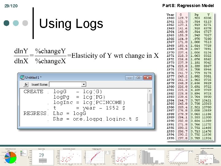
Part 8: Regression Model 29/120 Using Logs 29

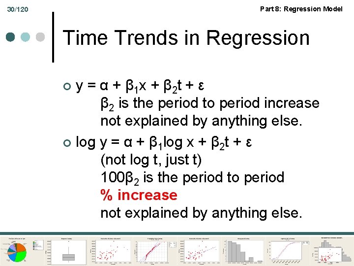
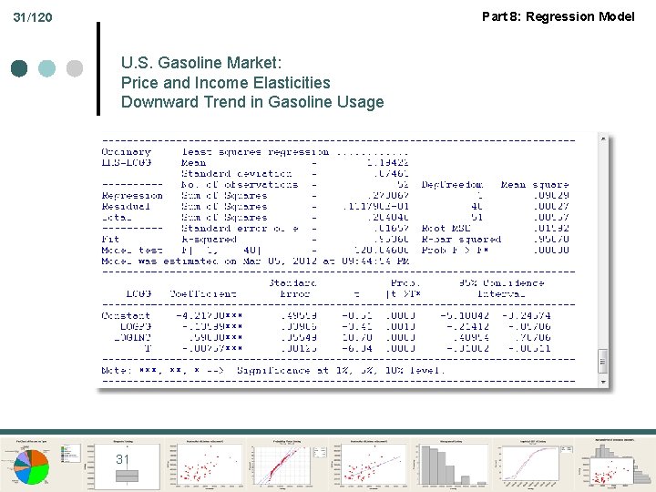
Part 8: Regression Model 30/120 Time Trends in Regression y = α + β 1 x + β 2 t + ε β 2 is the period to period increase not explained by anything else. ¢ log y = α + β 1 log x + β 2 t + ε (not log t, just t) 100β 2 is the period to period % increase not explained by anything else. ¢

Part 8: Regression Model 31/120 U. S. Gasoline Market: Price and Income Elasticities Downward Trend in Gasoline Usage 31

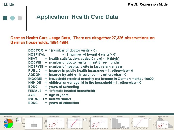
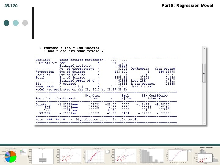
Part 8: Regression Model 32/120 Application: Health Care Data German Health Care Usage Data, There altogether 27, 326 observations on German households, 1984 -1994. DOCTOR = 1(number of doctor visits > 0) HOSPITAL = 1(number of hospital visits > 0) HSAT = health satisfaction, coded 0 (low) - 10 (high) DOCVIS = number of doctor visits in last three months HOSPVIS = number of hospital visits in last calendar year PUBLIC = insured in public health insurance = 1; otherwise = 0 ADDON = insured by add-on insurance = 1; otherswise = 0 INCOME = household nominal monthly net income in German marks / 10000. HHKIDS = children under age 16 in the household = 1; otherwise = 0 EDUC = years of schooling FEMALE = 1(female headed household) AGE = age in years MARRIED = marital status EDUC = years of education

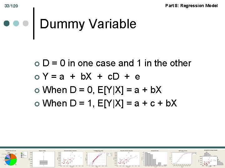
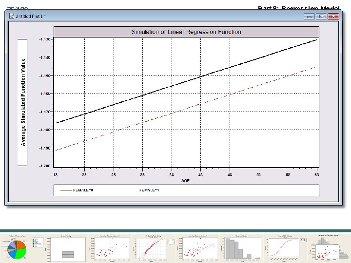
Part 8: Regression Model 33/120 Dummy Variable D = 0 in one case and 1 in the other ¢ Y = a + b. X + c. D + e ¢ When D = 0, E[Y|X] = a + b. X ¢ When D = 1, E[Y|X] = a + c + b. X ¢

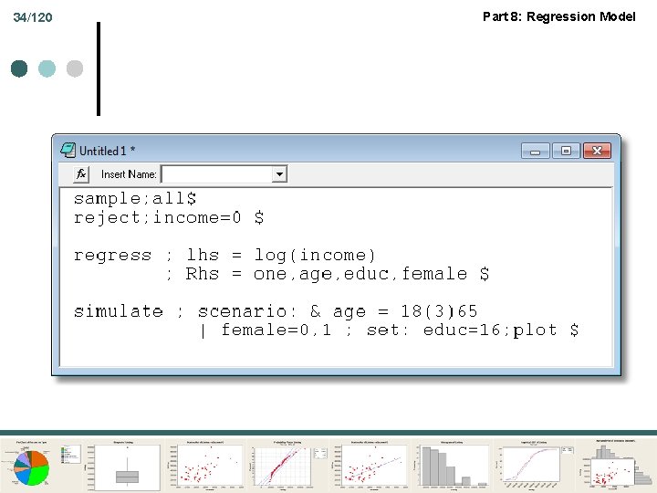
34/120 Part 8: Regression Model

35/120 Part 8: Regression Model

36/120 Part 8: Regression Model

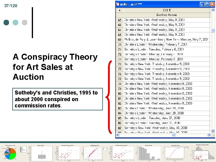
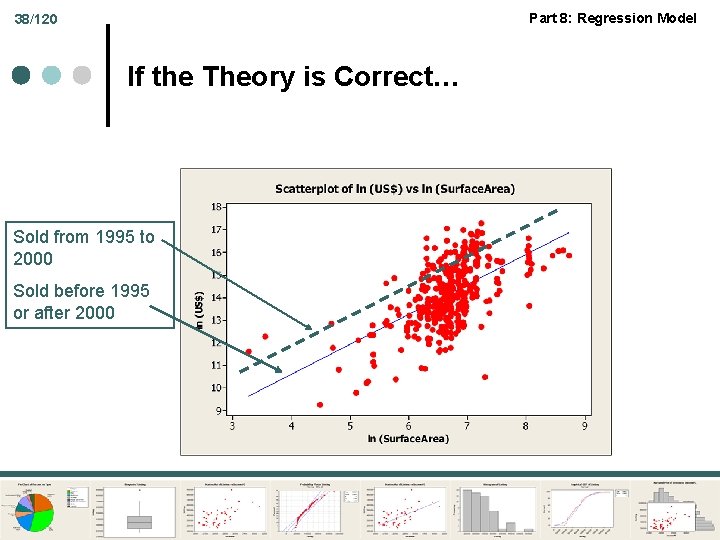
37/120 A Conspiracy Theory for Art Sales at Auction Sotheby’s and Christies, 1995 to about 2000 conspired on commission rates. Part 8: Regression Model

Part 8: Regression Model 38/120 If the Theory is Correct… Sold from 1995 to 2000 Sold before 1995 or after 2000

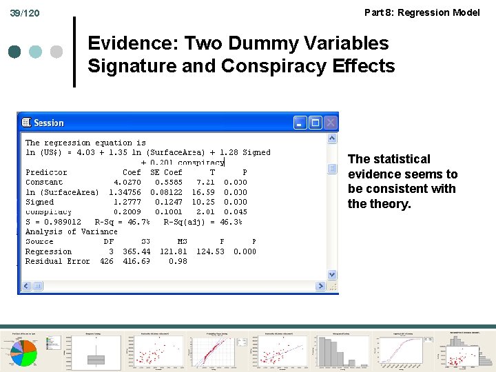
39/120 Part 8: Regression Model Evidence: Two Dummy Variables Signature and Conspiracy Effects The statistical evidence seems to be consistent with theory.

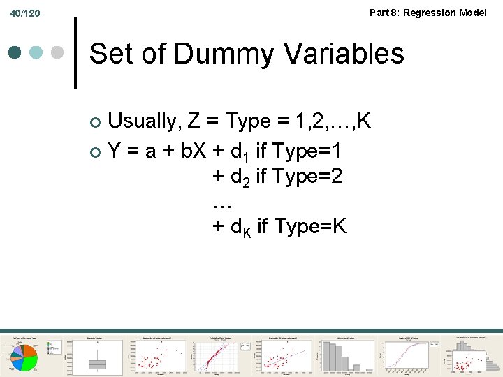
Part 8: Regression Model 40/120 Set of Dummy Variables Usually, Z = Type = 1, 2, …, K ¢ Y = a + b. X + d 1 if Type=1 + d 2 if Type=2 … + d. K if Type=K ¢

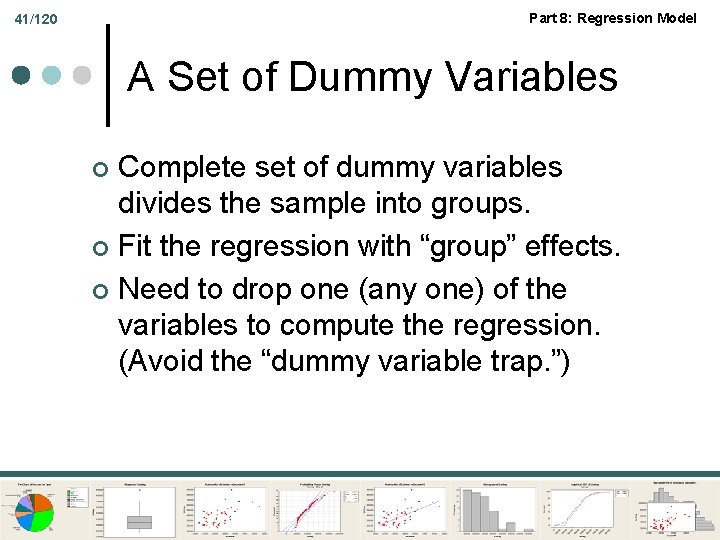
Part 8: Regression Model 41/120 A Set of Dummy Variables Complete set of dummy variables divides the sample into groups. ¢ Fit the regression with “group” effects. ¢ Need to drop one (any one) of the variables to compute the regression. (Avoid the “dummy variable trap. ”) ¢

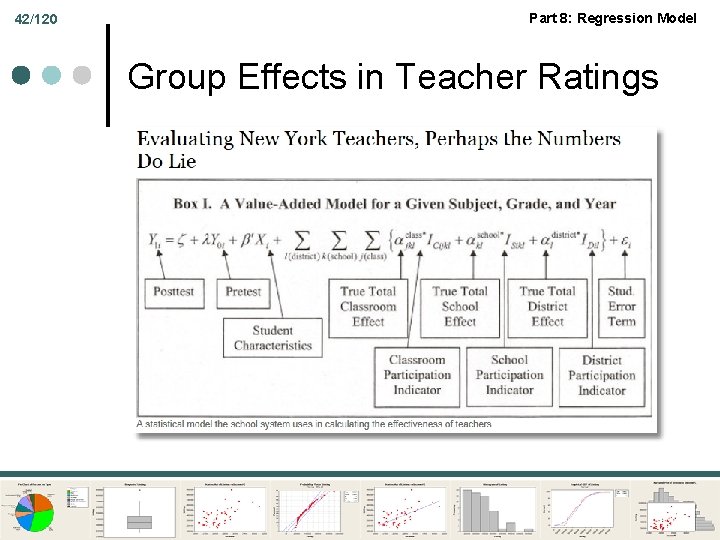
42/120 Part 8: Regression Model Group Effects in Teacher Ratings

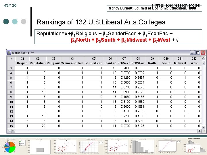
43/120 Part 8: Regression Model Nancy Burnett: Journal of Economic Education, 1998 Rankings of 132 U. S. Liberal Arts Colleges Reputation=α+β 1 Religious + β 2 Gender. Econ + β 3 Econ. Fac + β 4 North + β 5 South + β 6 Midwest + β 7 West + ε

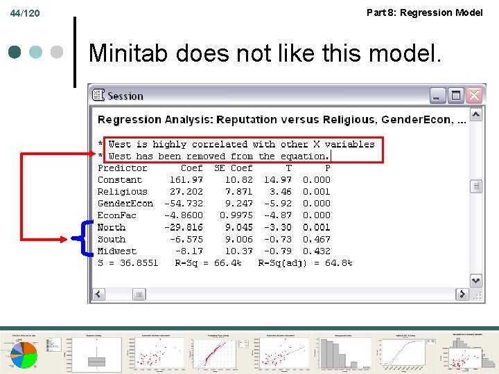
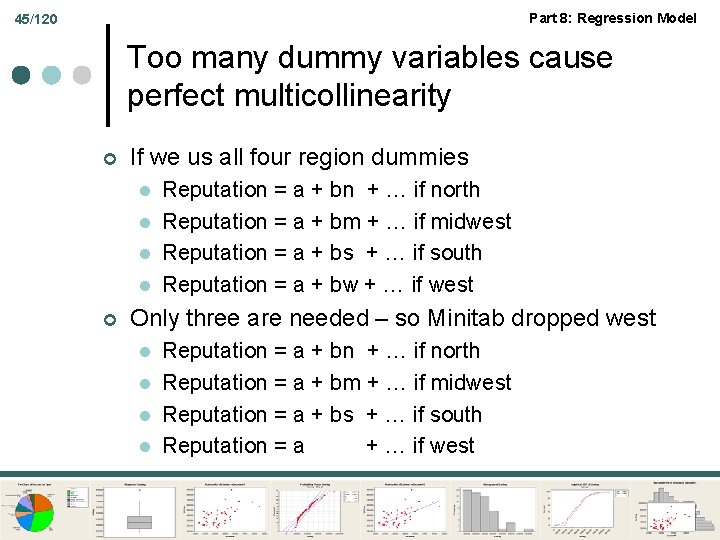
44/120 Part 8: Regression Model Minitab does not like this model.

Part 8: Regression Model 45/120 Too many dummy variables cause perfect multicollinearity ¢ If we us all four region dummies l l ¢ Reputation = a + bn + … if north Reputation = a + bm + … if midwest Reputation = a + bs + … if south Reputation = a + bw + … if west Only three are needed – so Minitab dropped west l l Reputation = a + bn + … if north Reputation = a + bm + … if midwest Reputation = a + bs + … if south Reputation = a + … if west

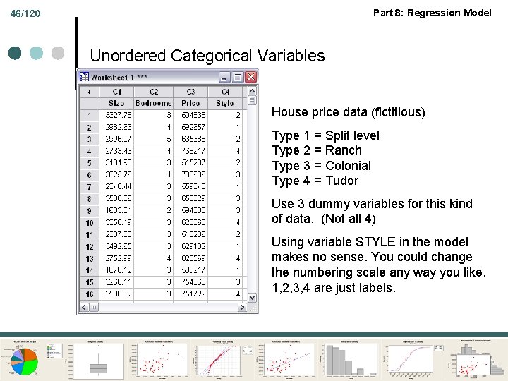
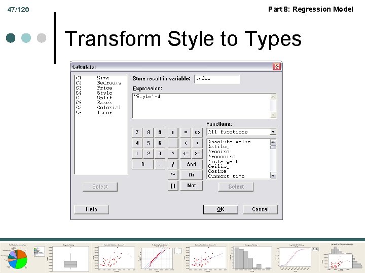
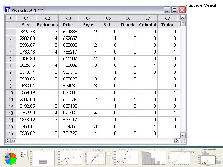
Part 8: Regression Model 46/120 Unordered Categorical Variables House price data (fictitious) Type 1 = Split level Type 2 = Ranch Type 3 = Colonial Type 4 = Tudor Use 3 dummy variables for this kind of data. (Not all 4) Using variable STYLE in the model makes no sense. You could change the numbering scale any way you like. 1, 2, 3, 4 are just labels.

47/120 Part 8: Regression Model Transform Style to Types

48/120 Part 8: Regression Model

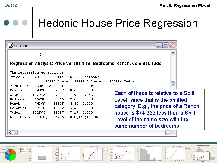
49/120 Part 8: Regression Model Hedonic House Price Regression Each of these is relative to a Split Level, since that is the omitted category. E. g. , the price of a Ranch house is $74, 369 less than a Split Level of the same size with the same number of bedrooms.

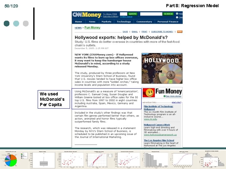
Part 8: Regression Model 50/120 We used Mc. Donald’s Per Capita

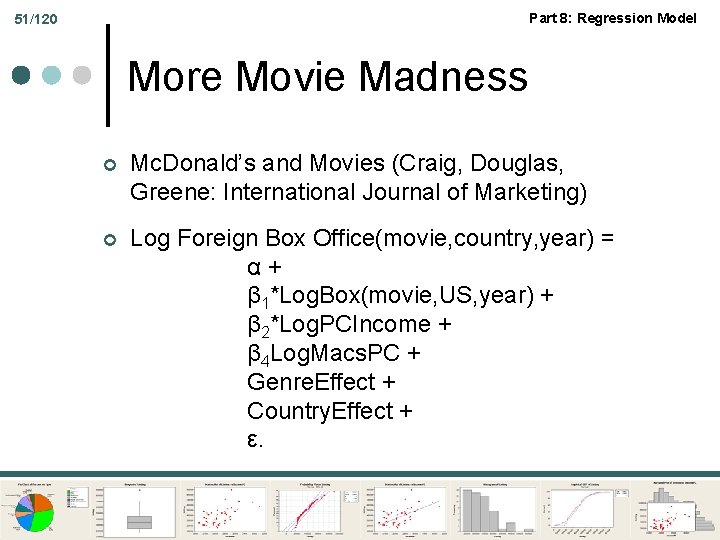
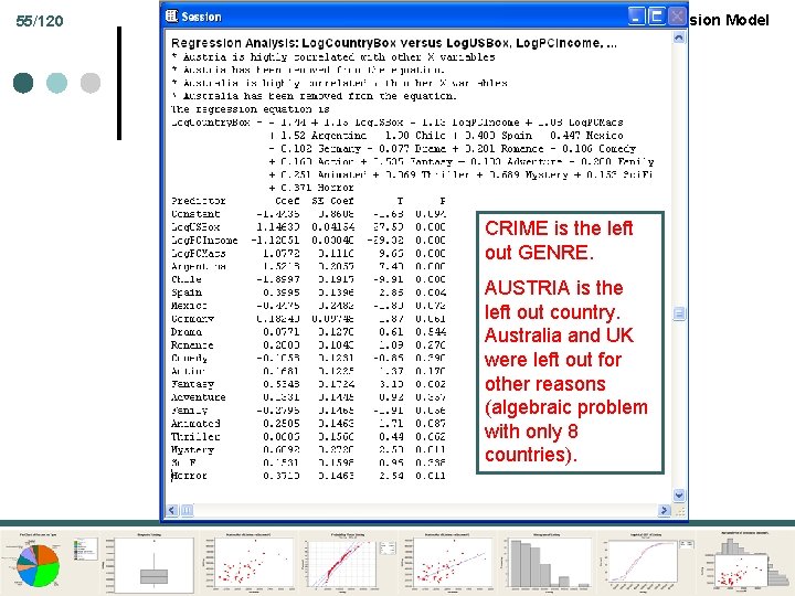
Part 8: Regression Model 51/120 More Movie Madness ¢ Mc. Donald’s and Movies (Craig, Douglas, Greene: International Journal of Marketing) ¢ Log Foreign Box Office(movie, country, year) = α+ β 1*Log. Box(movie, US, year) + β 2*Log. PCIncome + β 4 Log. Macs. PC + Genre. Effect + Country. Effect + ε.

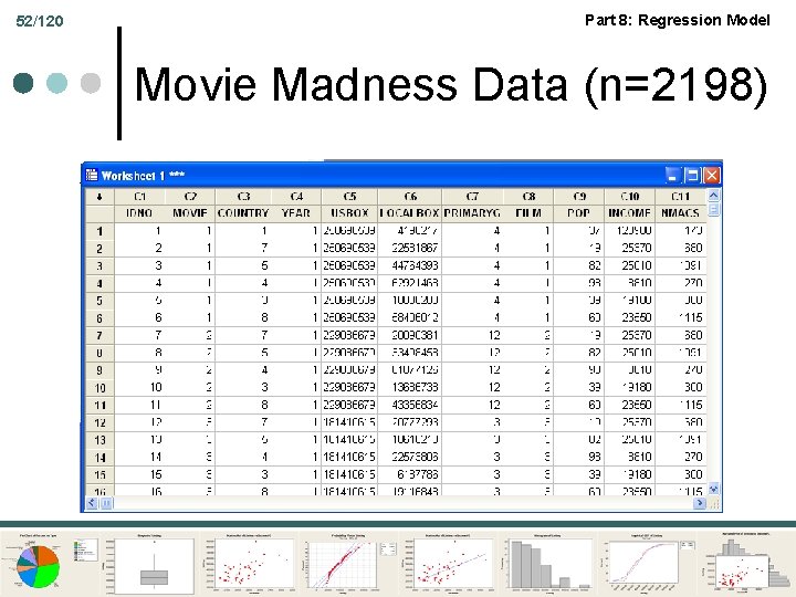
52/120 Part 8: Regression Model Movie Madness Data (n=2198)

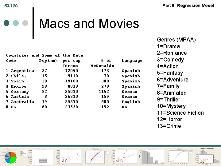
Part 8: Regression Model 53/120 Macs and Movies Countries and Some of the Data Code Pop(mm) per cap Income 1 Argentina 37 12090 2 Chile, 15 9110 3 Spain 39 19180 4 Mexico 98 8810 5 Germany 82 25010 6 Austria 8 26310 7 Australia 19 25370 8 UK 60 23550 # of Mc. Donalds 173 70 300 270 1152 159 680 1152 Language Spanish German English UK Genres (MPAA) 1=Drama 2=Romance 3=Comedy 4=Action 5=Fantasy 6=Adventure 7=Family 8=Animated 9=Thriller 10=Mystery 11=Science Fiction 12=Horror 13=Crime

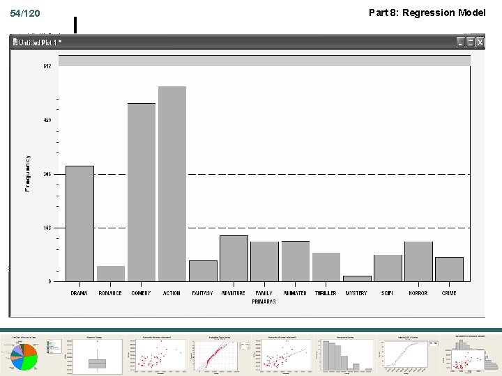
54/120 Part 8: Regression Model

55/120 Part 8: Regression Model CRIME is the left out GENRE. AUSTRIA is the left out country. Australia and UK were left out for other reasons (algebraic problem with only 8 countries).

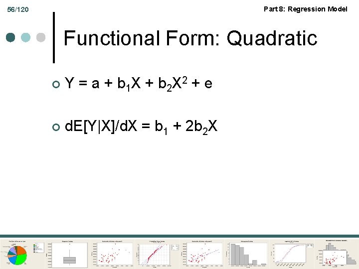
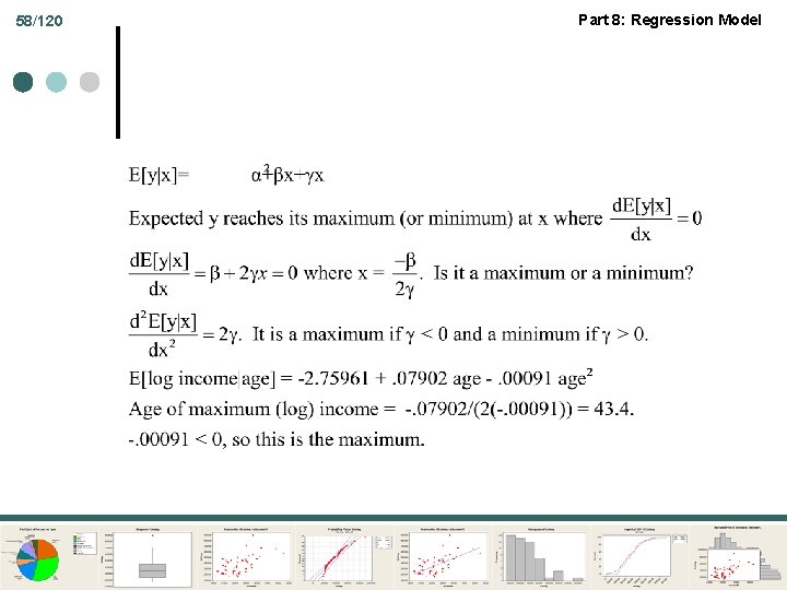
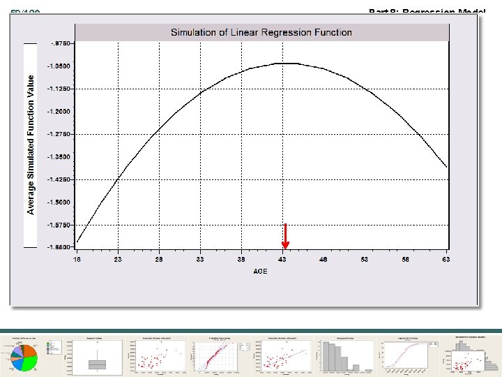
Part 8: Regression Model 56/120 Functional Form: Quadratic ¢ Y = a + b 1 X + b 2 X 2 + e ¢ d. E[Y|X]/d. X = b 1 + 2 b 2 X

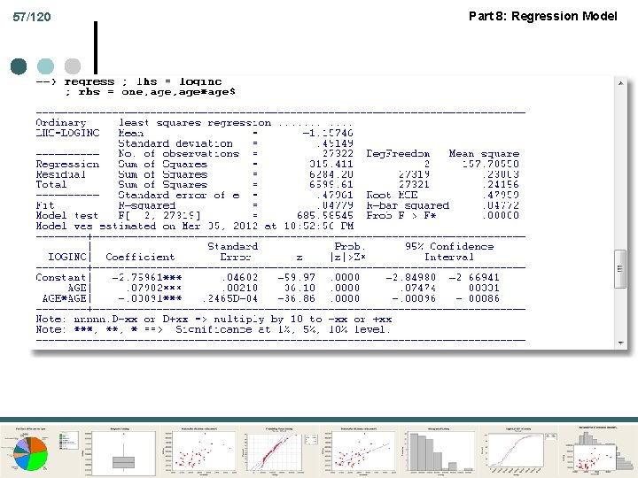
57/120 Part 8: Regression Model

58/120 Part 8: Regression Model

59/120 Part 8: Regression Model

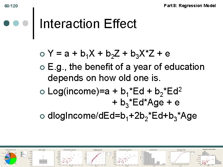
Part 8: Regression Model 60/120 Interaction Effect Y = a + b 1 X + b 2 Z + b 3 X*Z + e ¢ E. g. , the benefit of a year of education depends on how old one is. ¢ Log(income)=a + b 1*Ed + b 2*Ed 2 + b 3*Ed*Age + e ¢ dlog. Income/d. Ed=b 1+2 b 2*Ed+b 3*Age ¢

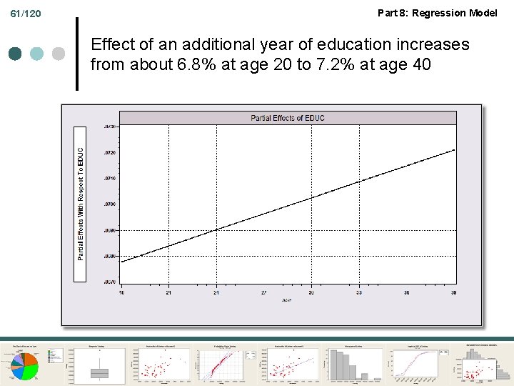
61/120 Part 8: Regression Model Effect of an additional year of education increases from about 6. 8% at age 20 to 7. 2% at age 40

Part 8: Regression Model Statistics and Data Analysis Properties of Least Squares

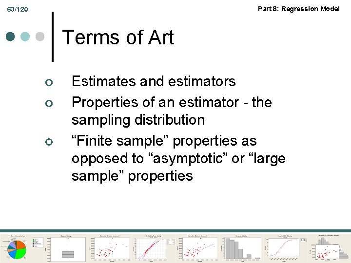
Part 8: Regression Model 63/120 Terms of Art ¢ ¢ ¢ Estimates and estimators Properties of an estimator - the sampling distribution “Finite sample” properties as opposed to “asymptotic” or “large sample” properties

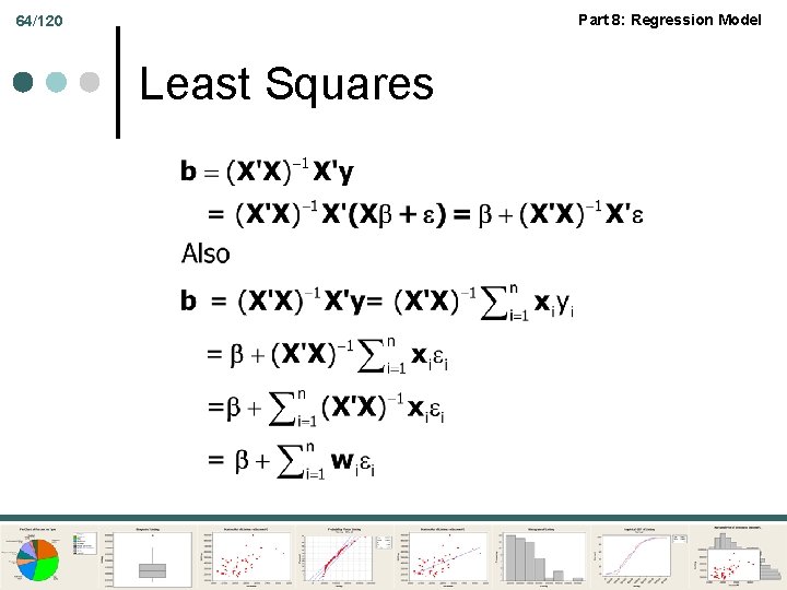
Part 8: Regression Model 64/120 Least Squares

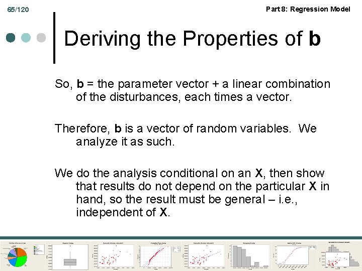
65/120 Part 8: Regression Model Deriving the Properties of b So, b = the parameter vector + a linear combination of the disturbances, each times a vector. Therefore, b is a vector of random variables. We analyze it as such. We do the analysis conditional on an X, then show that results do not depend on the particular X in hand, so the result must be general – i. e. , independent of X.

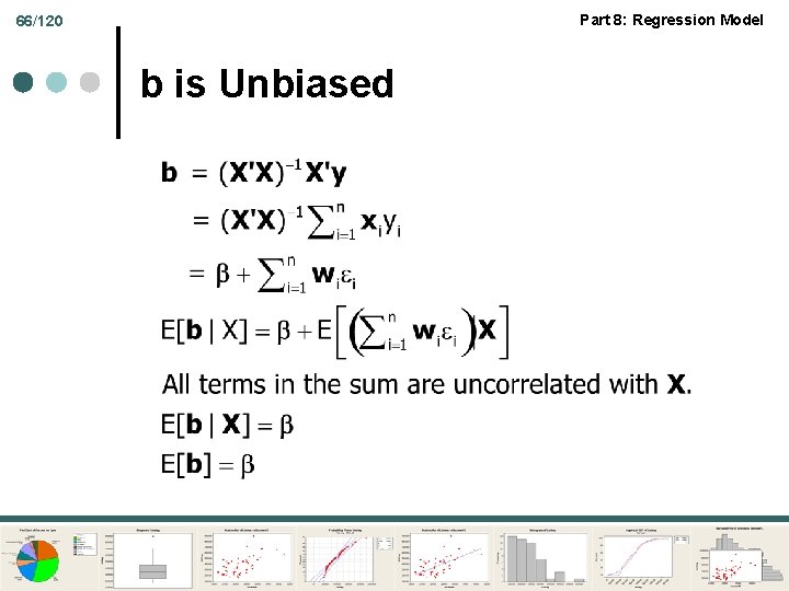
Part 8: Regression Model 66/120 b is Unbiased

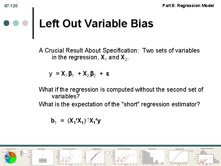
Part 8: Regression Model 67/120 Left Out Variable Bias A Crucial Result About Specification: Two sets of variables in the regression, X 1 and X 2. y = X 1 1 + X 2 2 + What if the regression is computed without the second set of variables? What is the expectation of the "short" regression estimator? b 1 = (X 1 X 1)-1 X 1 y

Part 8: Regression Model 68/120 The Left Out Variable Formula E[b 1] = 1 + (X 1 X 1)-1 X 1 X 2 2 The (truly) short regression estimator is biased. Application: Quantity = 1 Price + 2 Income + If you regress Quantity on Price and leave out Income. What do you get?

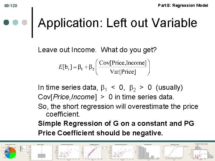
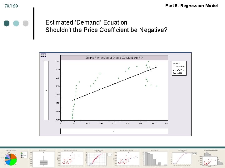
Part 8: Regression Model 69/120 Application: Left out Variable Leave out Income. What do you get? In time series data, 1 < 0, 2 > 0 (usually) Cov[Price, Income] > 0 in time series data. So, the short regression will overestimate the price coefficient. Simple Regression of G on a constant and PG Price Coefficient should be negative.

70/120 Part 8: Regression Model Estimated ‘Demand’ Equation Shouldn’t the Price Coefficient be Negative?

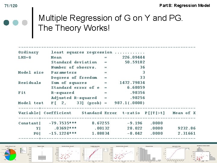
71/120 Part 8: Regression Model Multiple Regression of G on Y and PG. Theory Works! -----------------------------------Ordinary least squares regression. . . LHS=G Mean = 226. 09444 Standard deviation = 50. 59182 Number of observs. = 36 Model size Parameters = 3 Degrees of freedom = 33 Residuals Sum of squares = 1472. 79834 Standard error of e = 6. 68059 Fit R-squared =. 98356 Adjusted R-squared =. 98256 Model test F[ 2, 33] (prob) = 987. 1(. 0000) ----+------------------------------Variable| Coefficient Standard Error t-ratio P[|T|>t] Mean of X ----+------------------------------Constant| -79. 7535*** 8. 67255 -9. 196. 0000 Y|. 03692***. 00132 28. 022. 0000 9232. 86 PG| -15. 1224*** 1. 88034 -8. 042. 0000 2. 31661 ----+-------------------------------

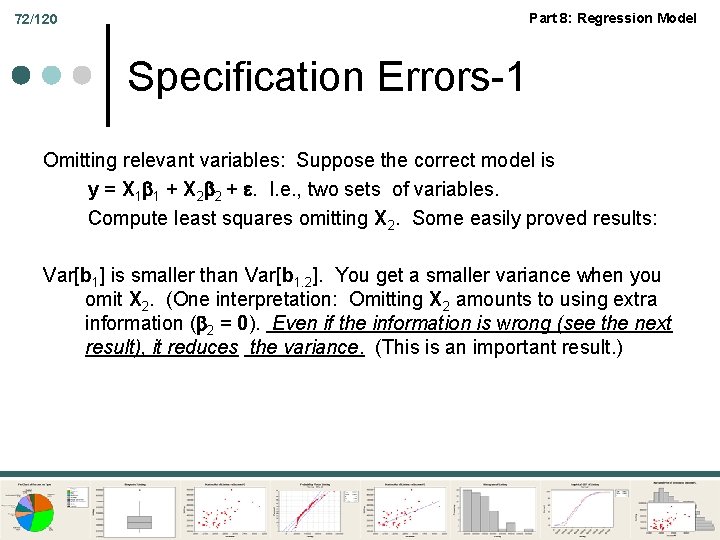
Part 8: Regression Model 72/120 Specification Errors-1 Omitting relevant variables: Suppose the correct model is y = X 1 1 + X 2 2 + . I. e. , two sets of variables. Compute least squares omitting X 2. Some easily proved results: Var[b 1] is smaller than Var[b 1. 2]. You get a smaller variance when you omit X 2. (One interpretation: Omitting X 2 amounts to using extra information ( 2 = 0). Even if the information is wrong (see the next result), it reduces the variance. (This is an important result. )

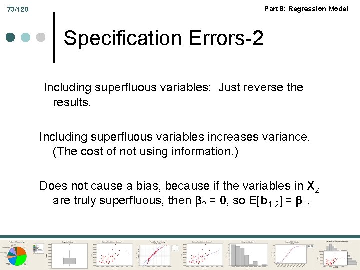
Part 8: Regression Model 73/120 Specification Errors-2 Including superfluous variables: Just reverse the results. Including superfluous variables increases variance. (The cost of not using information. ) Does not cause a bias, because if the variables in X 2 are truly superfluous, then 2 = 0, so E[b 1. 2] = 1.

Part 8: Regression Model Inference and Regression Estimating Var[b|X]

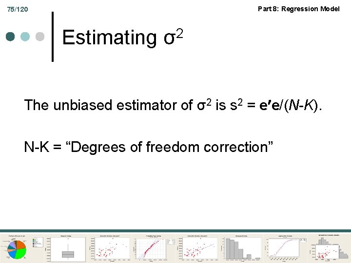
Part 8: Regression Model 75/120 Estimating σ2 The unbiased estimator of σ2 is s 2 = e e/(N-K). N-K = “Degrees of freedom correction”

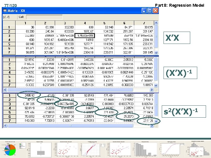
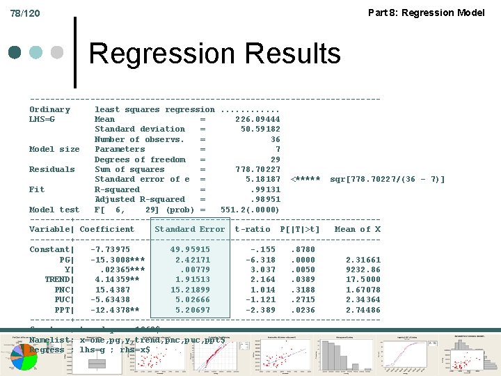
Part 8: Regression Model 76/120 Var[b|X] Estimating the Covariance Matrix for b|X The true covariance matrix is 2 (X’X)-1 The natural estimator is s 2(X’X)-1 “Standard errors” of the individual coefficients are the square roots of the diagonal elements.

77/120 Part 8: Regression Model X’X (X’X)-1 s 2(X’X)-1

Part 8: Regression Model 78/120 Regression Results -----------------------------------Ordinary least squares regression. . . LHS=G Mean = 226. 09444 Standard deviation = 50. 59182 Number of observs. = 36 Model size Parameters = 7 Degrees of freedom = 29 Residuals Sum of squares = 778. 70227 Standard error of e = 5. 18187 <***** sqr[778. 70227/(36 – 7)] Fit R-squared =. 99131 Adjusted R-squared =. 98951 Model test F[ 6, 29] (prob) = 551. 2(. 0000) ----+------------------------------Variable| Coefficient Standard Error t-ratio P[|T|>t] Mean of X ----+------------------------------Constant| -7. 73975 49. 95915 -. 155. 8780 PG| -15. 3008*** 2. 42171 -6. 318. 0000 2. 31661 Y|. 02365***. 00779 3. 037. 0050 9232. 86 TREND| 4. 14359** 1. 91513 2. 164. 0389 17. 5000 PNC| 15. 4387 15. 21899 1. 014. 3188 1. 67078 PUC| -5. 63438 5. 02666 -1. 121. 2715 2. 34364 PPT| -12. 4378** 5. 20697 -2. 389. 0236 2. 74486 ----+------------------------------Create ; trend=year-1960$ Namelist; x=one, pg, y, trend, pnc, puc, ppt$ Regress ; lhs=g ; rhs=x$

Part 8: Regression Model Inference and Regression Not Perfect Collinearity

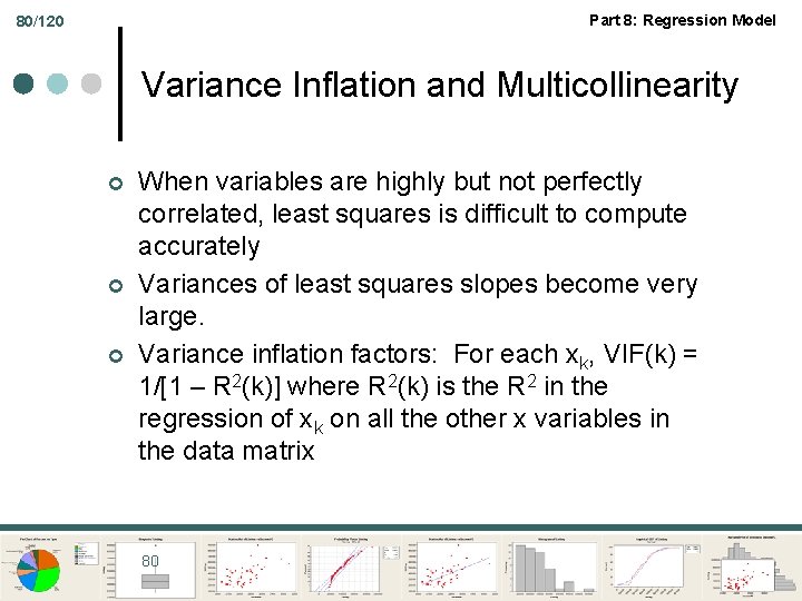
Part 8: Regression Model 80/120 Variance Inflation and Multicollinearity ¢ ¢ ¢ When variables are highly but not perfectly correlated, least squares is difficult to compute accurately Variances of least squares slopes become very large. Variance inflation factors: For each xk, VIF(k) = 1/[1 – R 2(k)] where R 2(k) is the R 2 in the regression of xk on all the other x variables in the data matrix 80

81/120 Part 8: Regression Model NIST Statistical Reference Data Sets – Accuracy Tests

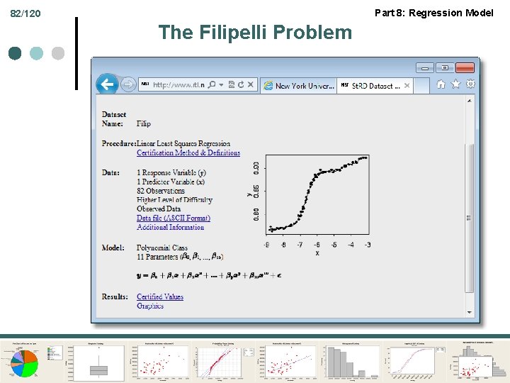
Part 8: Regression Model 82/120 The Filipelli Problem

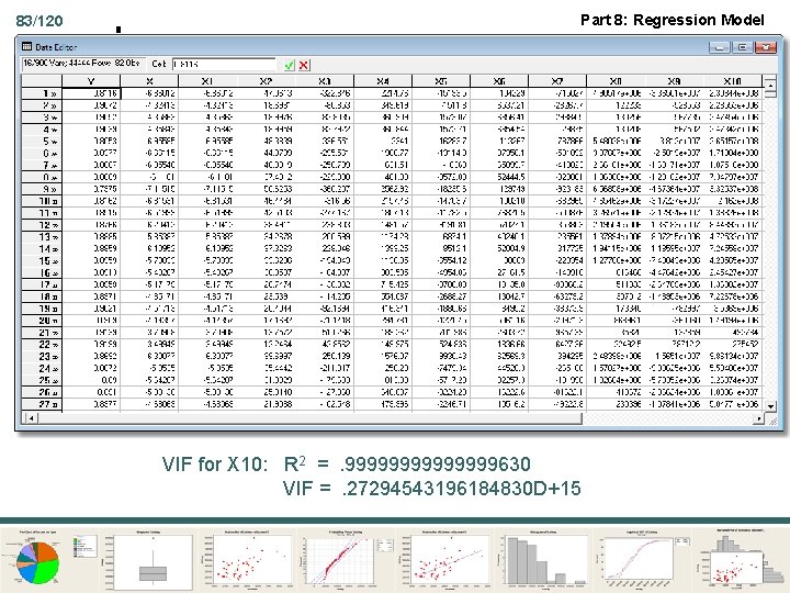
83/120 Part 8: Regression Model VIF for X 10: R 2 =. 9999999630 VIF =. 27294543196184830 D+15

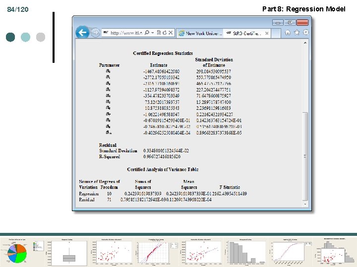
84/120 Part 8: Regression Model

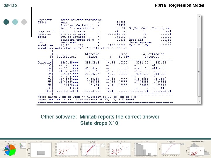
85/120 Part 8: Regression Model Other software: Minitab reports the correct answer Stata drops X 10

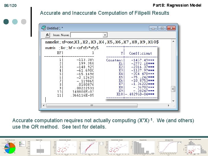
86/120 Part 8: Regression Model Accurate and Inaccurate Computation of Filipelli Results Accurate computation requires not actually computing (X’X)-1. We (and others) use the QR method. See text for details.

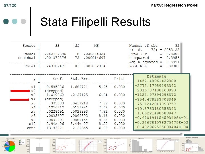
87/120 Part 8: Regression Model Stata Filipelli Results

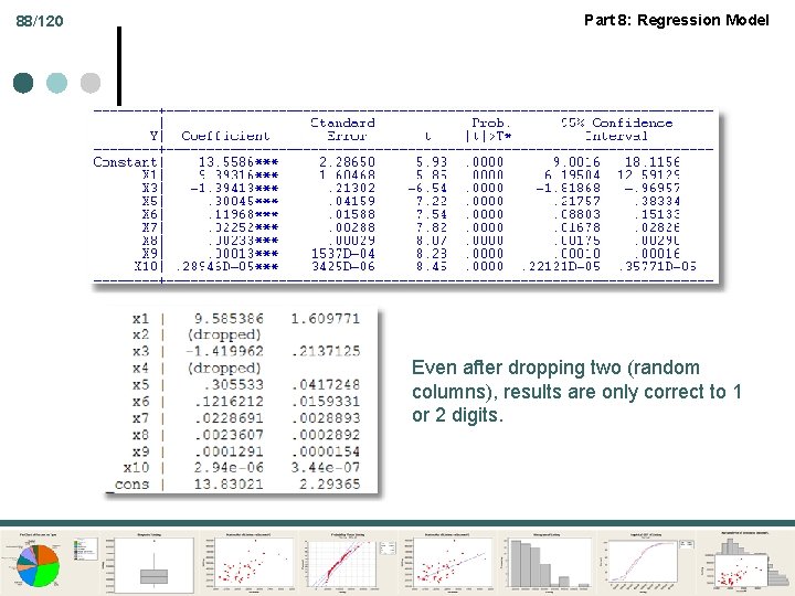
88/120 Part 8: Regression Model Even after dropping two (random columns), results are only correct to 1 or 2 digits.

Part 8: Regression Model Inference and Regression Testing Hypotheses

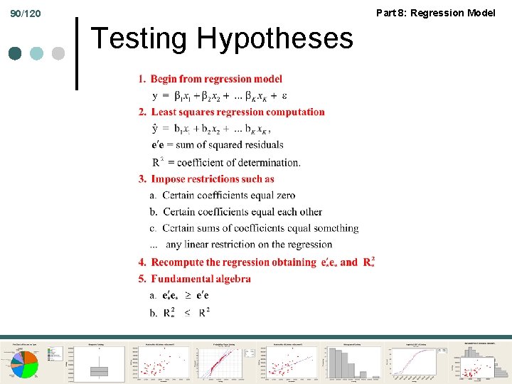
Part 8: Regression Model 90/120 Testing Hypotheses

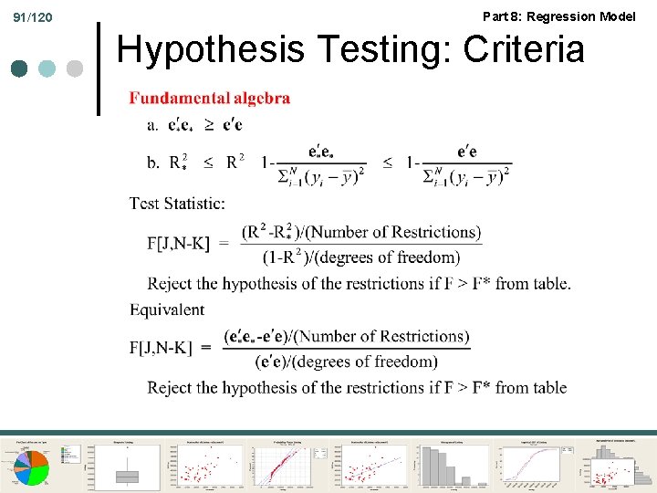
91/120 Part 8: Regression Model Hypothesis Testing: Criteria

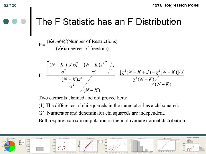
92/120 Part 8: Regression Model The F Statistic has an F Distribution

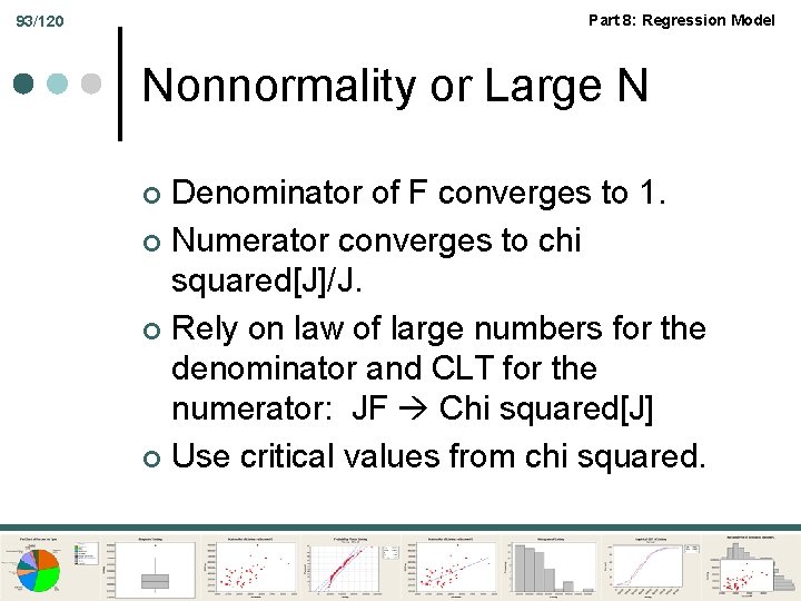
Part 8: Regression Model 93/120 Nonnormality or Large N Denominator of F converges to 1. ¢ Numerator converges to chi squared[J]/J. ¢ Rely on law of large numbers for the denominator and CLT for the numerator: JF Chi squared[J] ¢ Use critical values from chi squared. ¢

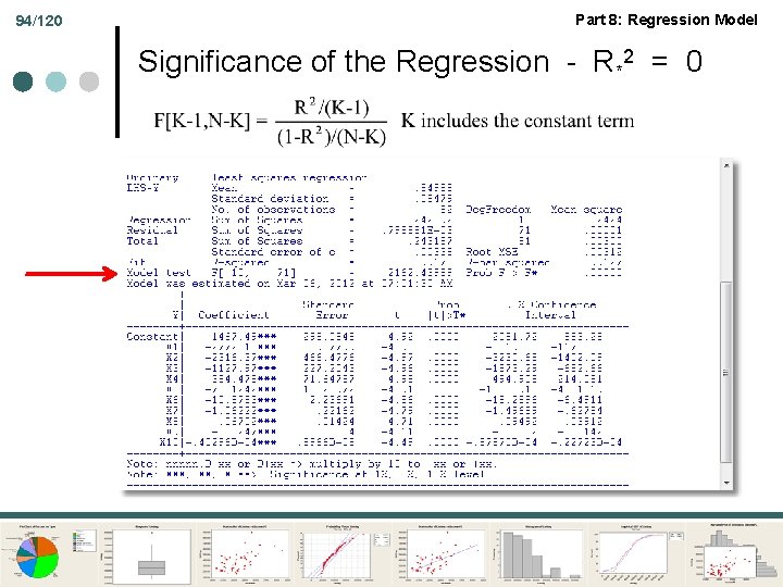
94/120 Part 8: Regression Model Significance of the Regression - R*2 = 0

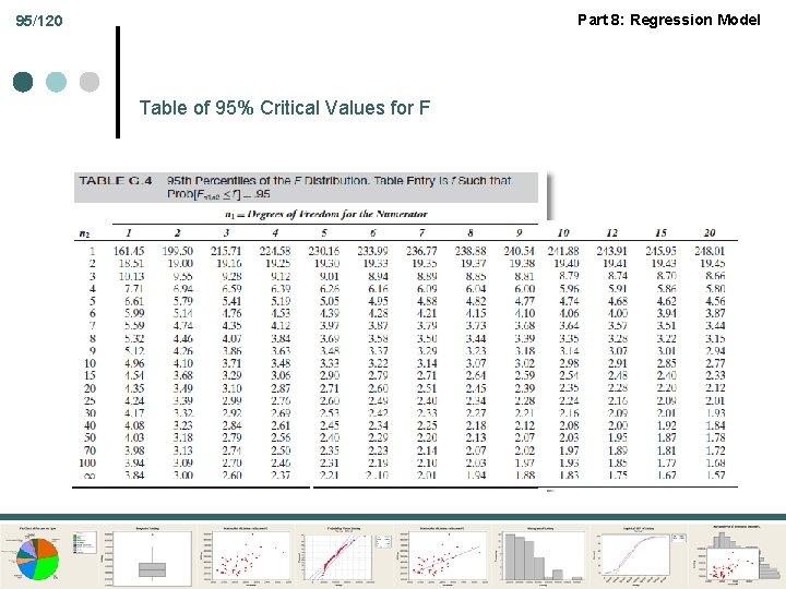
Part 8: Regression Model 95/120 Table of 95% Critical Values for F

96/120 Part 8: Regression Model

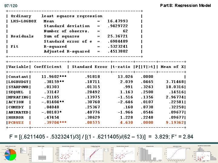
Part 8: Regression Model 97/120 +--------------------------+ | Ordinary least squares regression | | LHS=LOGBOX Mean = 16. 47993 | | Standard deviation =. 9429722 | | Number of observs. = 62 | | Residuals Sum of squares = 25. 36721 | | Standard error of e =. 6984489 | | Fit R-squared =. 5323241 | | Adjusted R-squared =. 4513802 | +--------------------------+ +--------------+--------+--------+-----+ |Variable| Coefficient | Standard Error |t-ratio |P[|T|>t]| Mean of X| +--------------+--------+--------+-----+ |Constant| 11. 9602***. 91818 13. 026. 0000 | |LOGBUDGT|. 38159**. 18711 2. 039. 0465 3. 71468| |STARPOWR|. 01303. 01315. 991. 3263 18. 0316| |SEQUEL |. 33147. 28492 1. 163. 2500. 14516| |MPRATING| -. 21185. 13975 -1. 516. 1356 2. 96774| |ACTION | -. 81404**. 30760 -2. 646. 0107. 22581| |COMEDY |. 04048. 25367. 160. 8738. 32258| |ANIMATED| -. 80183*. 40776 -1. 966. 0546. 09677| |HORROR |. 47454. 38629 1. 228. 2248. 09677| |PCBUZZ |. 39704***. 08575 4. 630. 0000 9. 19362| +----------------------------------+ F = [(. 6211405 -. 5323241)/3] / [(1 -. 6211405)/(62 – 13)] = 3. 829; F* = 2. 84