Online Social Networks and Media Link Analysis and

Online Social Networks and Media Link Analysis and Web Search

How to Organize the Web First try: Human curated Web directories Yahoo, DMOZ, Look. Smart

How to organize the web • Second try: Web Search – Information Retrieval investigates: • Find relevant docs in a small and trusted set e. g. , Newspaper articles, Patents, etc. (“needle-in-ahaystack”) • Limitation of keywords (synonyms, polysemy, etc) But: Web is huge, full of untrusted documents, random things, web spam, etc. § Everyone can create a web page of high production value § Rich diversity of people issuing queries § Dynamic and constantly-changing nature of web content

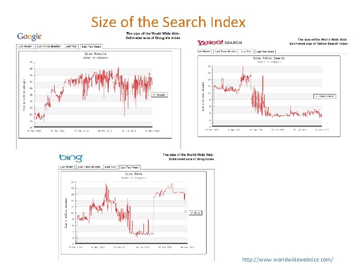
Size of the Search Index http: //www. worldwidewebsize. com/

How to organize the web • Third try (the Google era): using the web graph – Swift from relevance to authoritativeness – It is not only important that a page is relevant, but that it is also important on the web • For example, what kind of results would we like to get for the query “greek newspapers”?

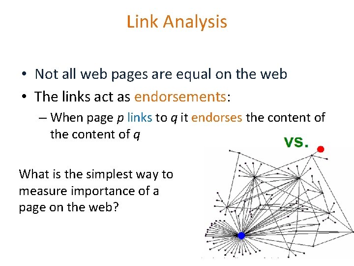
Link Analysis • Not all web pages are equal on the web • The links act as endorsements: – When page p links to q it endorses the content of q What is the simplest way to measure importance of a page on the web?

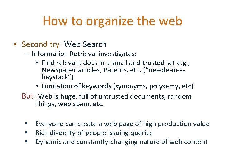
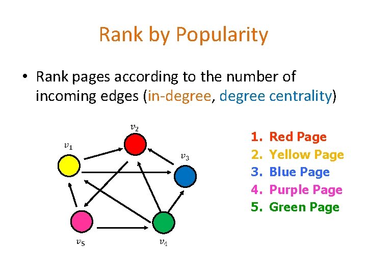
Rank by Popularity • Rank pages according to the number of incoming edges (in-degree, degree centrality) 1. 2. 3. 4. 5. Red Page Yellow Page Blue Page Purple Page Green Page

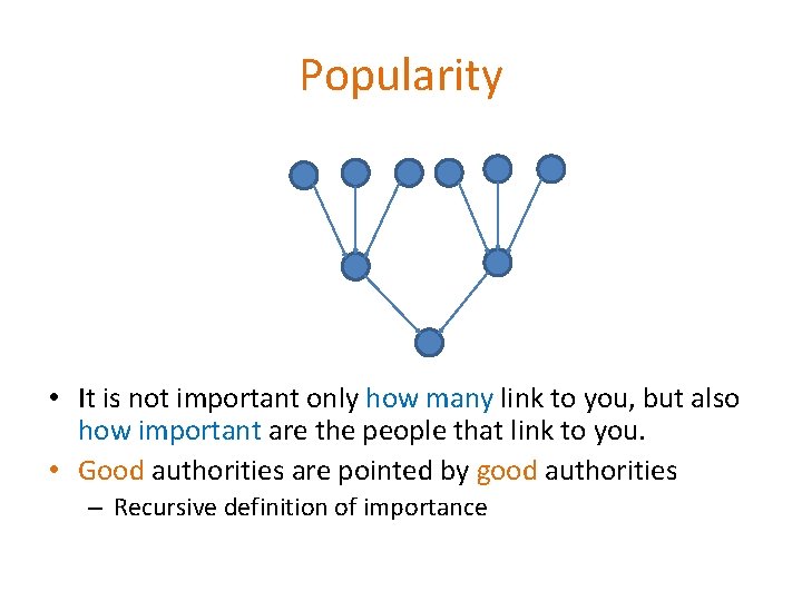
Popularity • It is not important only how many link to you, but also how important are the people that link to you. • Good authorities are pointed by good authorities – Recursive definition of importance

THE PAGERANK ALGORITHM

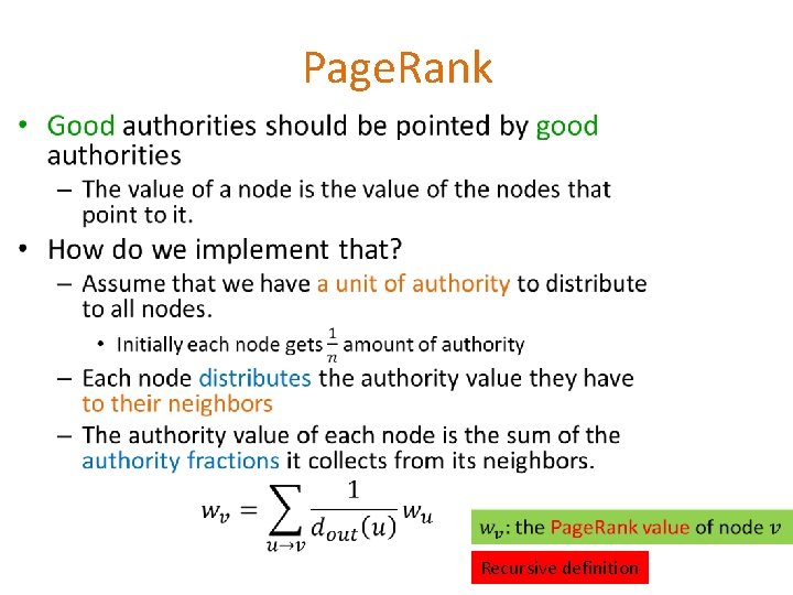
Page. Rank • Recursive definition

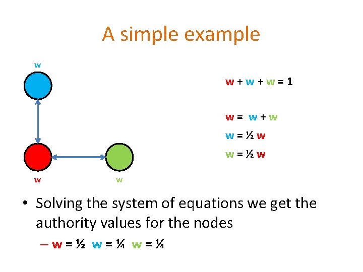
A simple example w w+w+w=1 w= w+w w=½w w w • Solving the system of equations we get the authority values for the nodes –w=½ w=¼

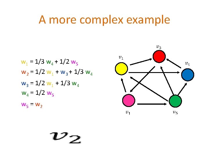
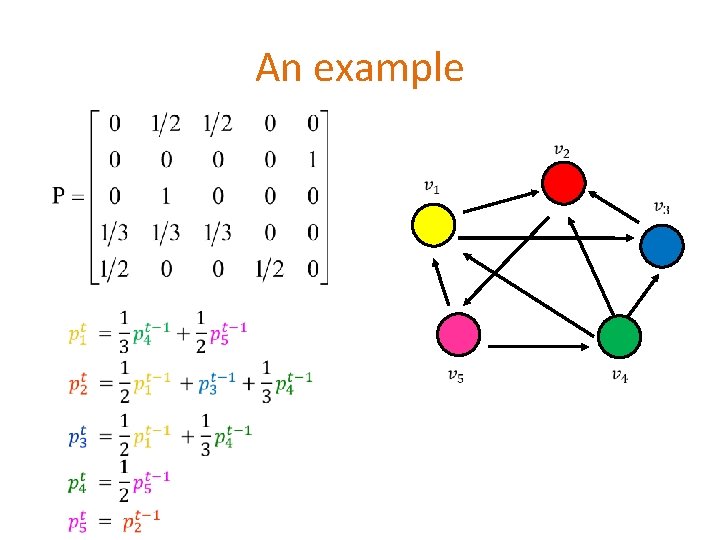
A more complex example w 1 = 1/3 w 4 + 1/2 w 5 w 2 = 1/2 w 1 + w 3 + 1/3 w 4 w 3 = 1/2 w 1 + 1/3 w 4 = 1/2 w 5 = w 2

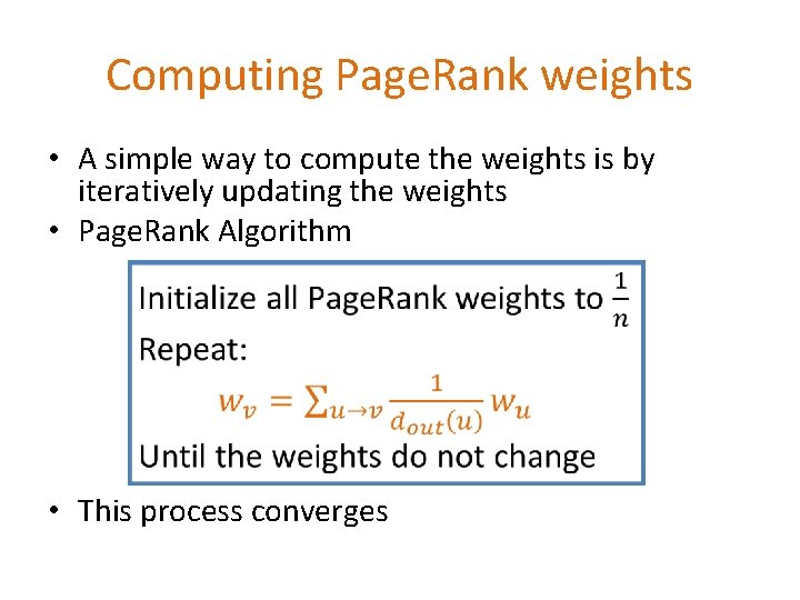
Computing Page. Rank weights • A simple way to compute the weights is by iteratively updating the weights • Page. Rank Algorithm • This process converges

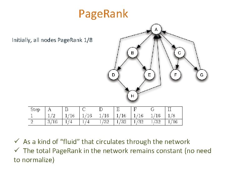
Page. Rank Initially, all nodes Page. Rank 1/8 ü As a kind of “fluid” that circulates through the network ü The total Page. Rank in the network remains constant (no need to normalize)

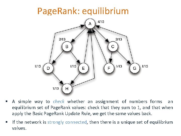
Page. Rank: equilibrium § A simple way to check whether an assignment of numbers forms an equilibrium set of Page. Rank values: check that they sum to 1, and that when apply the Basic Page. Rank Update Rule, we get the same values back. § If the network is strongly connected, then there is a unique set of equilibrium values.

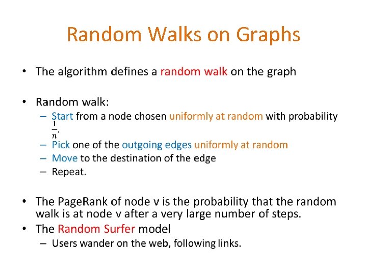
Random Walks on Graphs •

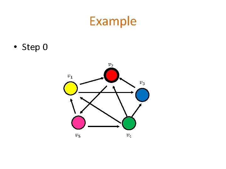
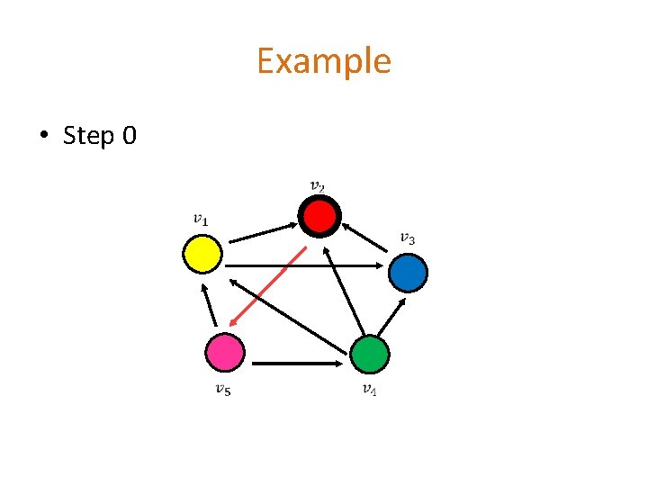
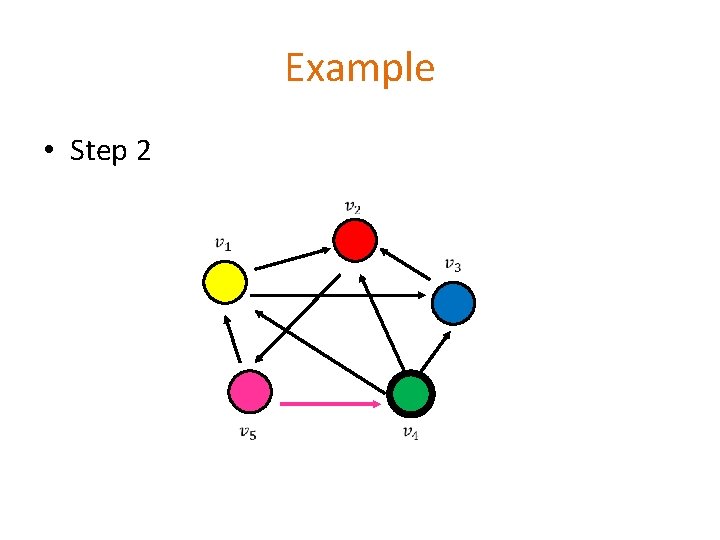
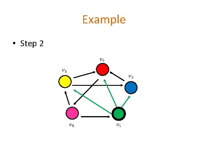
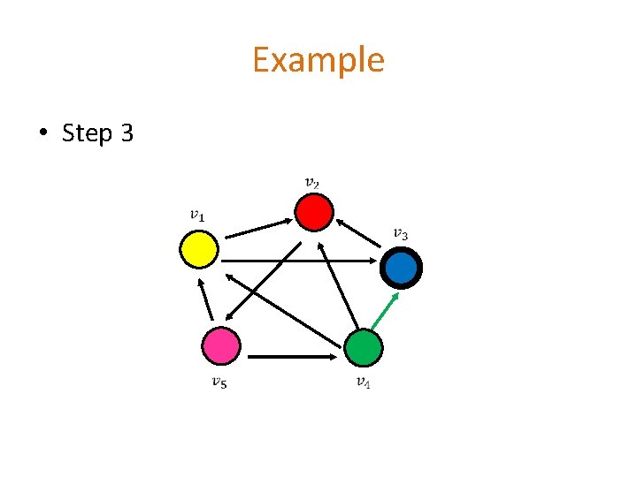
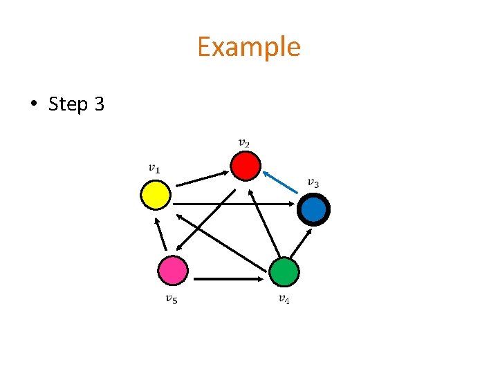
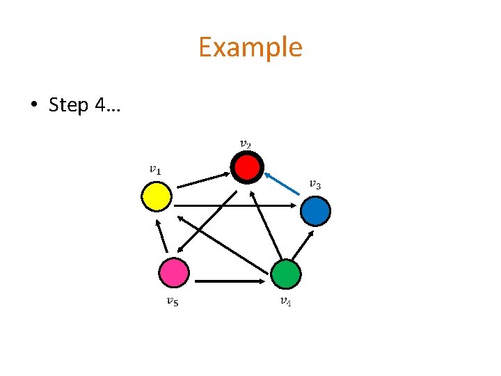
Example • Step 0

Example • Step 0

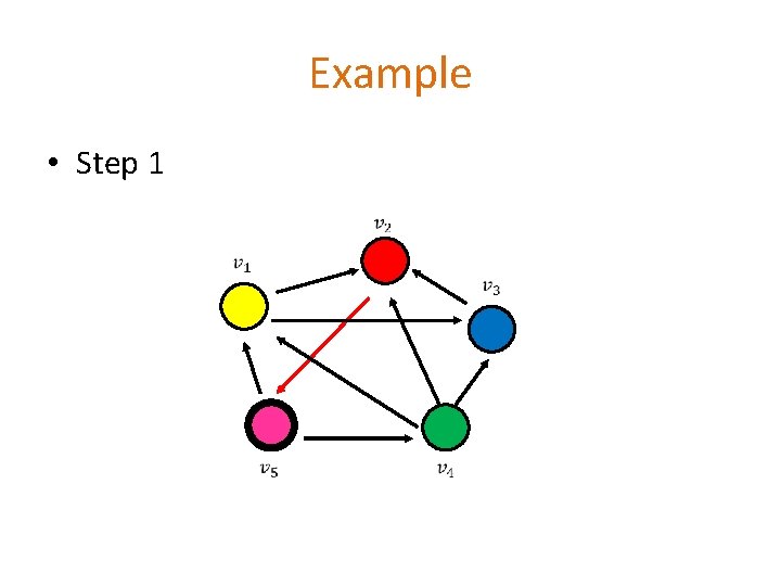
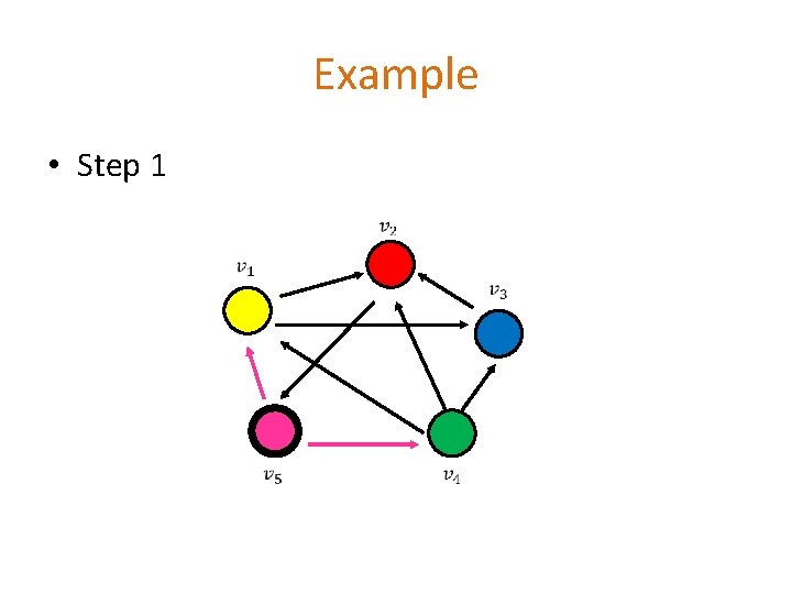
Example • Step 1

Example • Step 1

Example • Step 2

Example • Step 2

Example • Step 3

Example • Step 3

Example • Step 4…

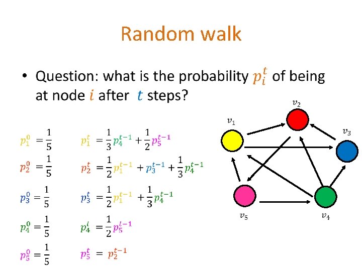
Random walk •

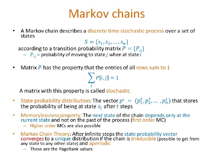
Markov chains •

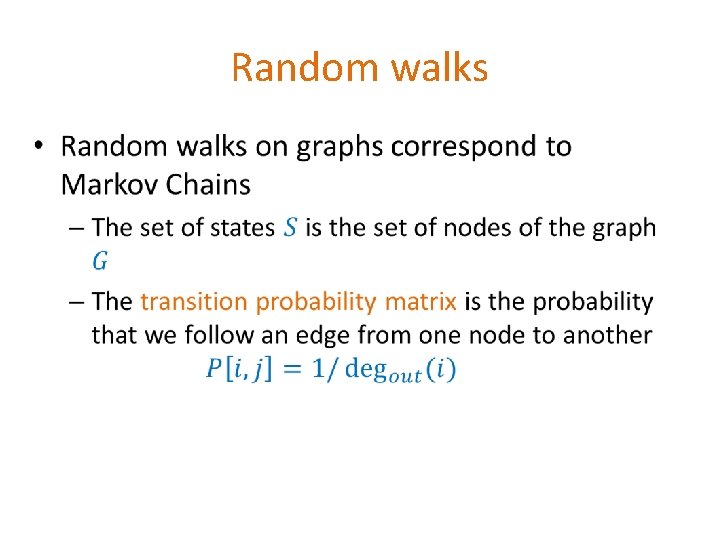
Random walks •

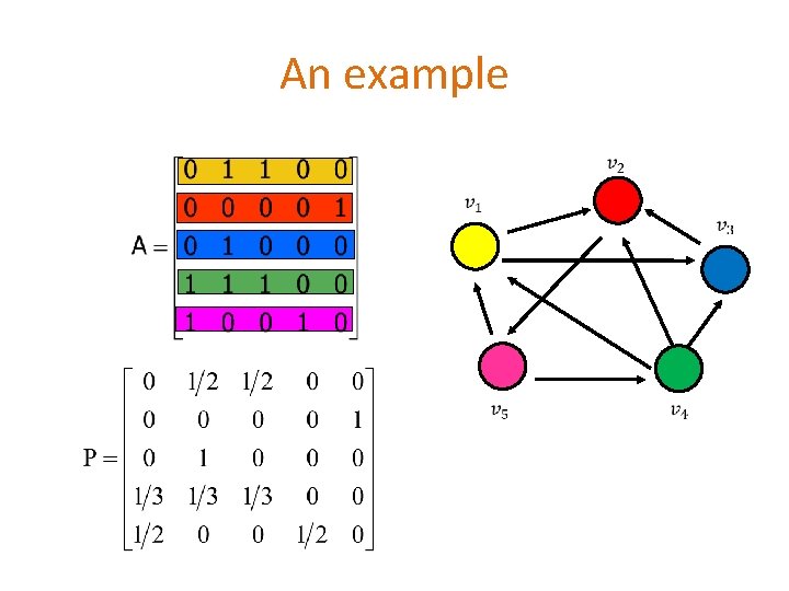
An example

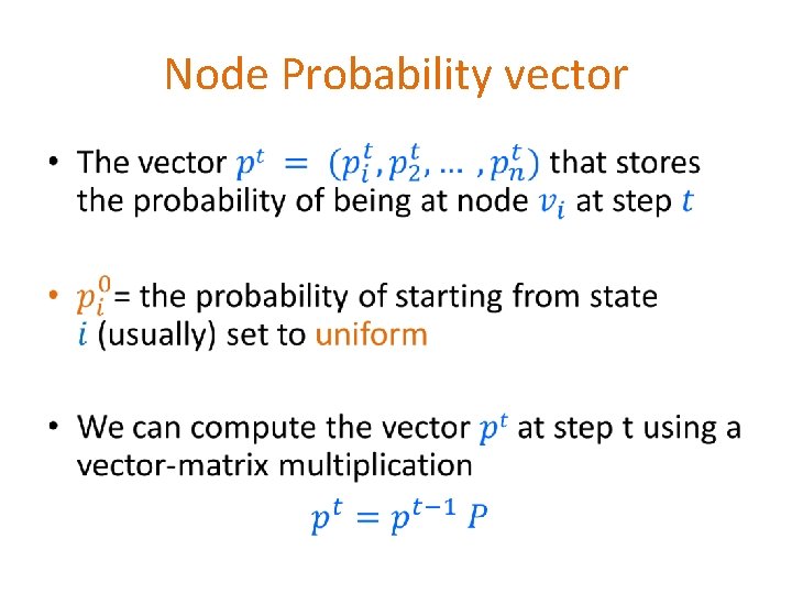
Node Probability vector •

An example

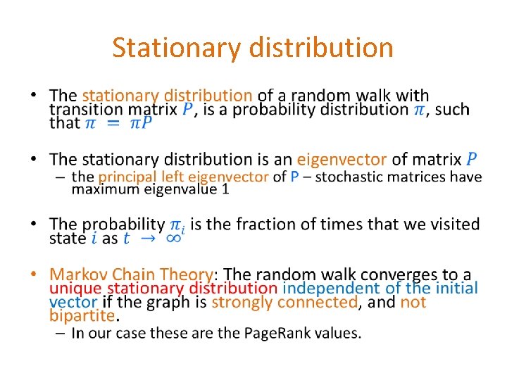
Stationary distribution •

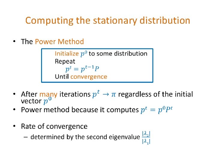
Computing the stationary distribution •

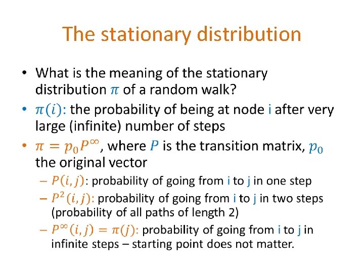
The stationary distribution •

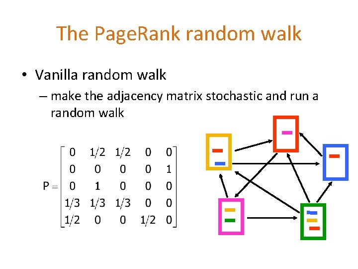
The Page. Rank random walk • Vanilla random walk – make the adjacency matrix stochastic and run a random walk

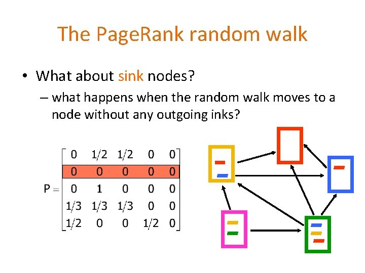
The Page. Rank random walk • What about sink nodes? – what happens when the random walk moves to a node without any outgoing inks?

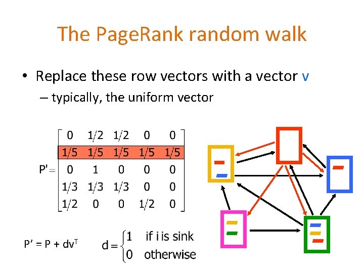
The Page. Rank random walk • Replace these row vectors with a vector v – typically, the uniform vector P’ = P + dv. T

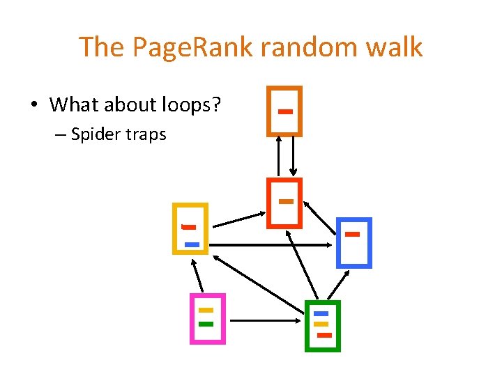
The Page. Rank random walk • What about loops? – Spider traps

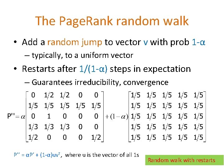
The Page. Rank random walk • Add a random jump to vector v with prob 1 -α – typically, to a uniform vector • Restarts after 1/(1 -α) steps in expectation – Guarantees irreducibility, convergence P’’ = αP’ + (1 -α)uv. T, where u is the vector of all 1 s Random walk with restarts

Page. Rank algorithm [BP 98] • 1. 2. 3. 4. 5. Red Page Purple Page Yellow Page Blue Page Green Page

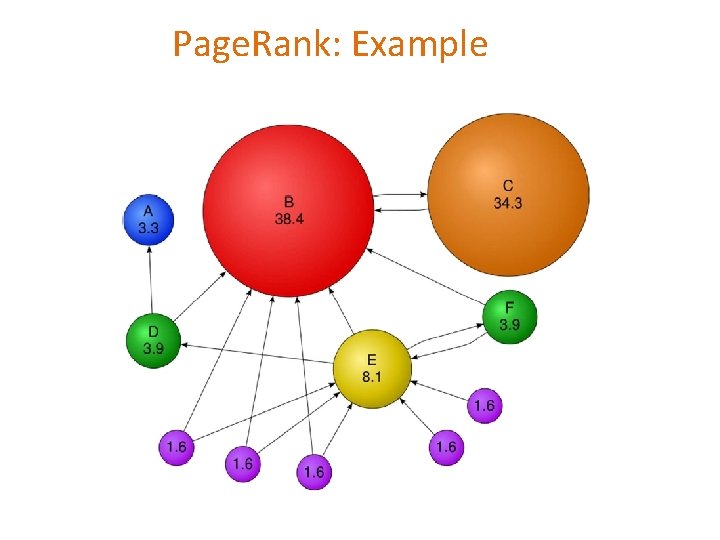
Page. Rank: Example

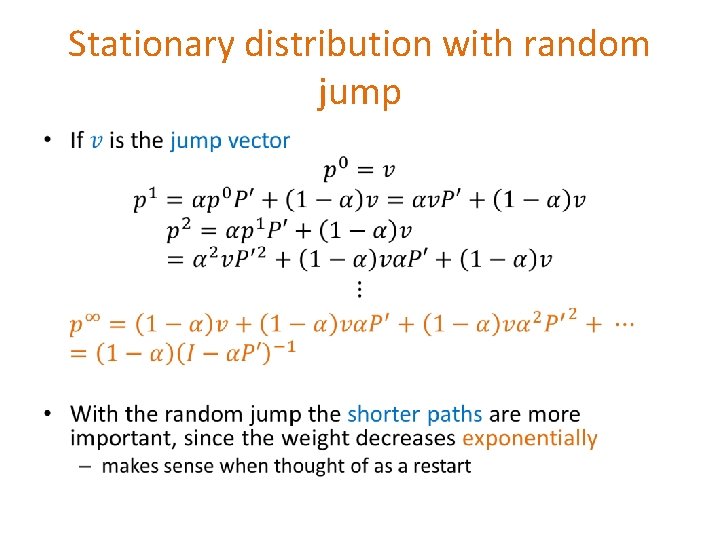
Stationary distribution with random jump •

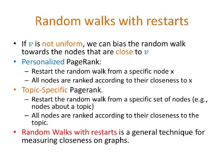
Random walks with restarts •

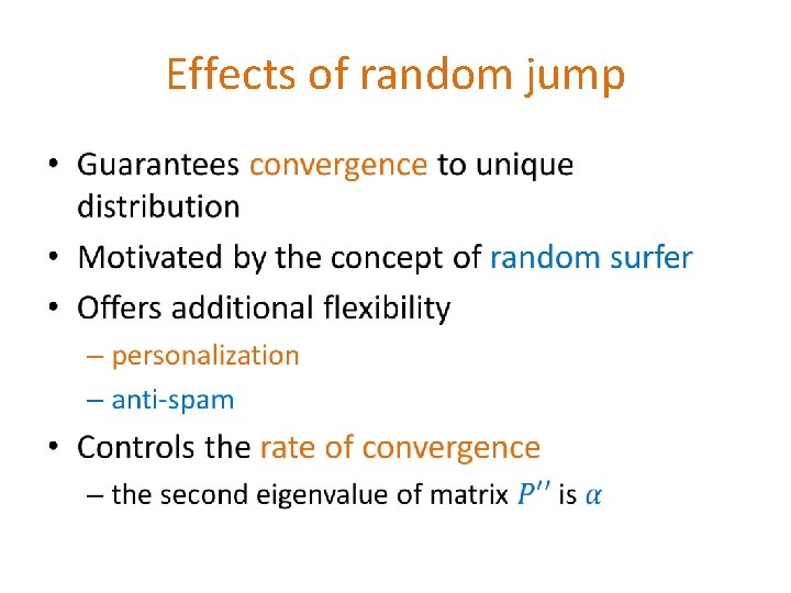
Effects of random jump •

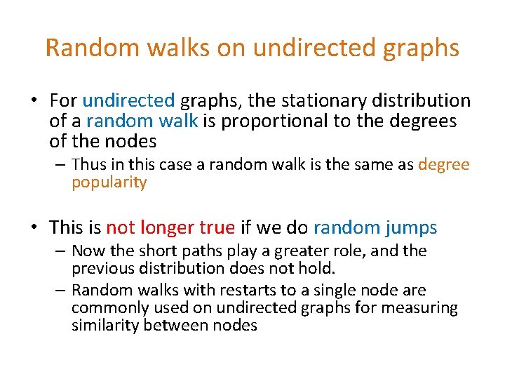
Random walks on undirected graphs • For undirected graphs, the stationary distribution of a random walk is proportional to the degrees of the nodes – Thus in this case a random walk is the same as degree popularity • This is not longer true if we do random jumps – Now the short paths play a greater role, and the previous distribution does not hold. – Random walks with restarts to a single node are commonly used on undirected graphs for measuring similarity between nodes

Page. Rank implementation •

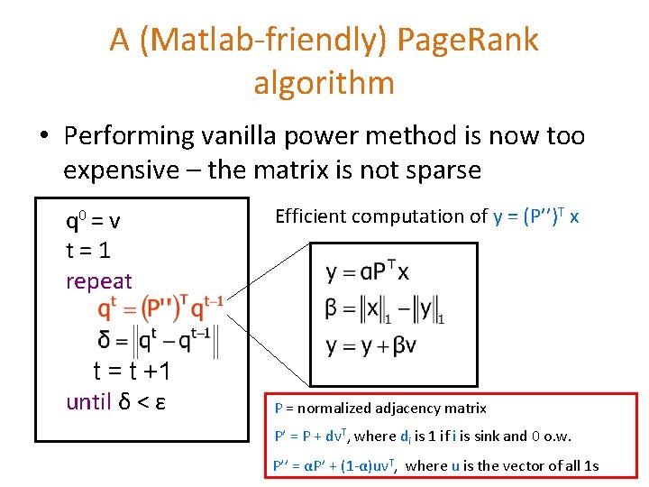
A (Matlab-friendly) Page. Rank algorithm • Performing vanilla power method is now too expensive – the matrix is not sparse q 0 = Efficient computation of y = (P’’)T x t = t +1 until δ < ε P = normalized adjacency matrix v t=1 repeat P’ = P + dv. T, where di is 1 if i is sink and 0 o. w. P’’ = αP’ + (1 -α)uv. T, where u is the vector of all 1 s

Page. Rank history • Huge advantage for Google in the early days – It gave a way to get an idea for the value of a page, which was useful in many different ways • Put an order to the web. – After a while it became clear that the anchor text was probably more important for ranking – Also, link spam became a new (dark) art • Flood of research – – Numerical analysis got rejuvenated Huge number of variations Efficiency became a great issue. Huge number of applications in different fields • Random walk is often referred to as Page. Rank.

THE HITS ALGORITHM

The HITS algorithm • Another algorithm proposed around the same time as Page. Rank for using the hyperlinks to rank pages – Kleinberg: then an intern at IBM Almaden – IBM never made anything out of it

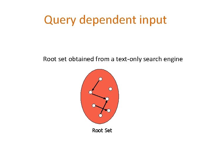
Query dependent input Root set obtained from a text-only search engine Root Set

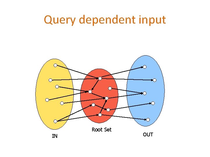
Query dependent input Root Set IN OUT

Query dependent input Root Set IN OUT

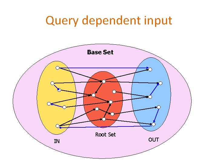
Query dependent input Base Set Root Set IN OUT

Hubs and Authorities [K 98] • Authority is not necessarily transferred directly between authorities • Pages have double identity – hub identity – authority identity • Good hubs point to good authorities • Good authorities are pointed by good hubs authorities

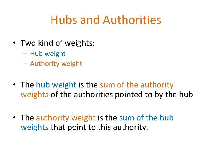
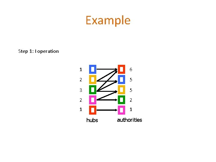
Hubs and Authorities • Two kind of weights: – Hub weight – Authority weight • The hub weight is the sum of the authority weights of the authorities pointed to by the hub • The authority weight is the sum of the hub weights that point to this authority.

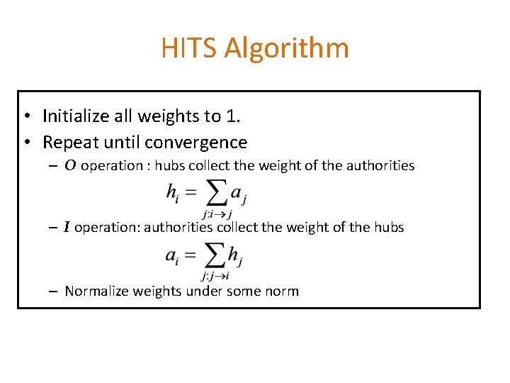
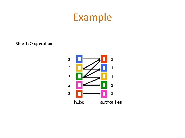
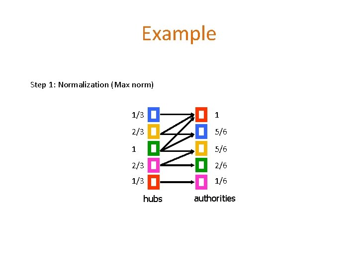
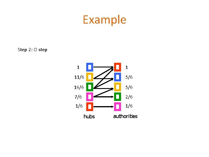
HITS Algorithm • Initialize all weights to 1. • Repeat until convergence – O operation : hubs collect the weight of the authorities – I operation: authorities collect the weight of the hubs – Normalize weights under some norm

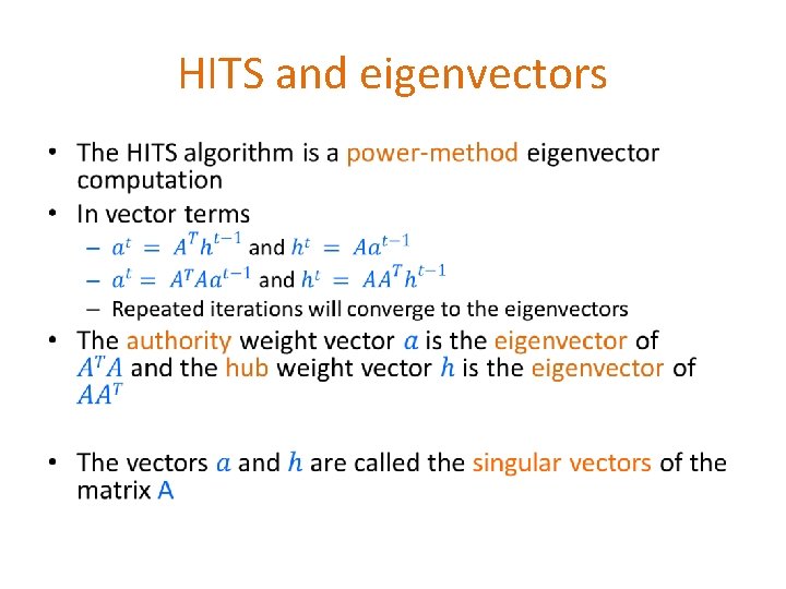
HITS and eigenvectors •

Singular Value Decomposition [n×r] [r×n] • r : rank of matrix A • σ1≥ σ2≥ … ≥σr : singular values (square roots of eig-vals AAT, ATA) • : left singular vectors (eig-vectors of AAT) • : right singular vectors (eig-vectors of ATA)

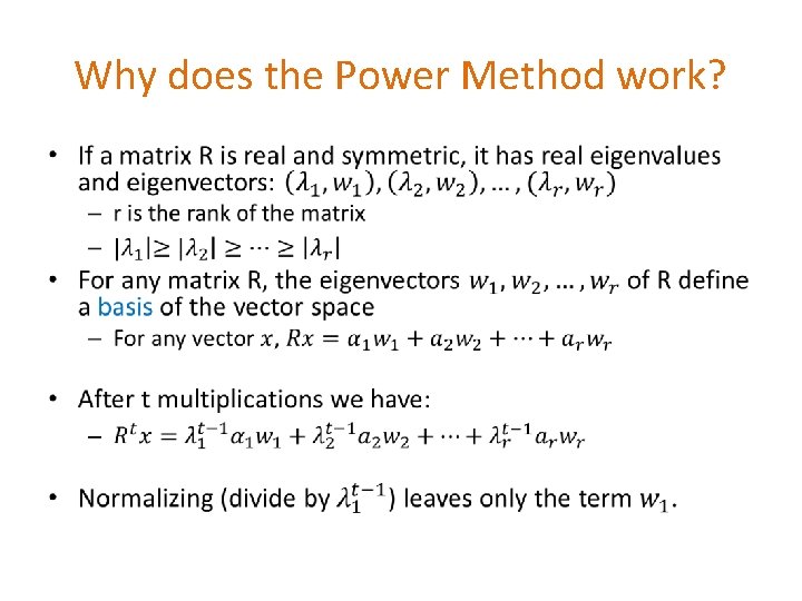
Why does the Power Method work? •

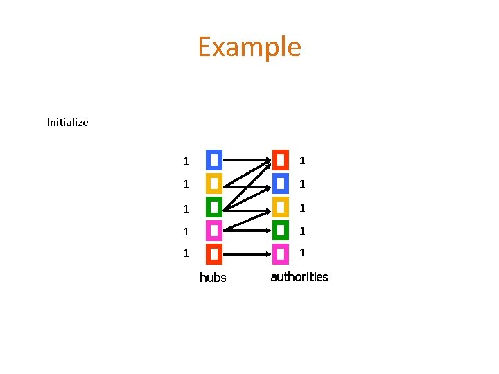
Example Initialize 1 1 1 1 1 hubs authorities

Example Step 1: O operation 1 1 2 1 3 1 2 1 1 1 hubs authorities

Example Step 1: I operation 1 6 2 5 3 5 2 2 1 1 hubs authorities

Example Step 1: Normalization (Max norm) 1/3 1 2/3 5/6 1 5/6 2/3 2/6 1/3 1/6 hubs authorities

Example Step 2: O step 1 1 11/6 5/6 16/6 5/6 7/6 2/6 1/6 hubs authorities

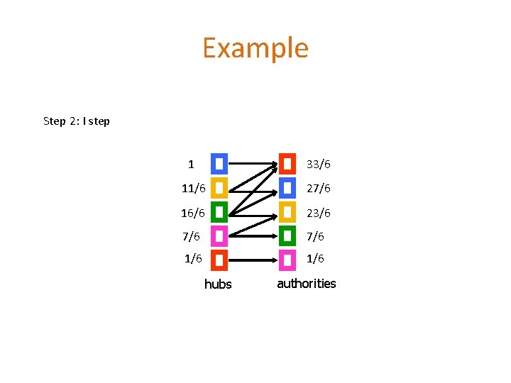
Example Step 2: I step 1 33/6 11/6 27/6 16/6 23/6 7/6 1/6 hubs authorities

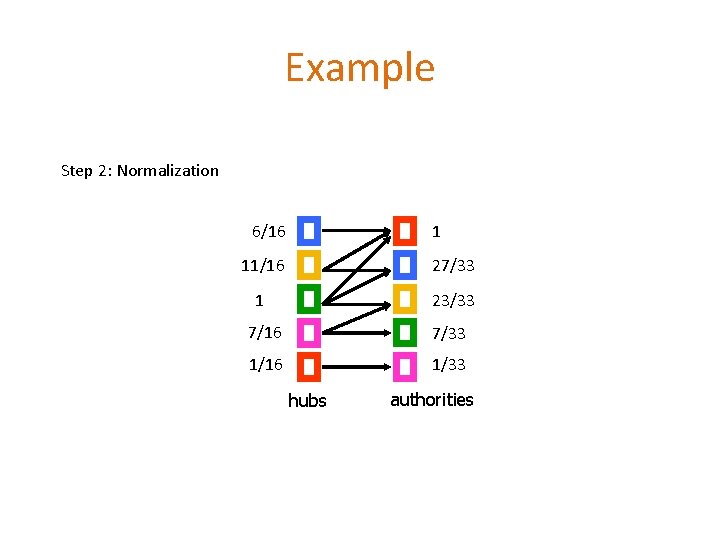
Example Step 2: Normalization 6/16 1 11/16 27/33 1 23/33 7/16 7/33 1/16 1/33 hubs authorities

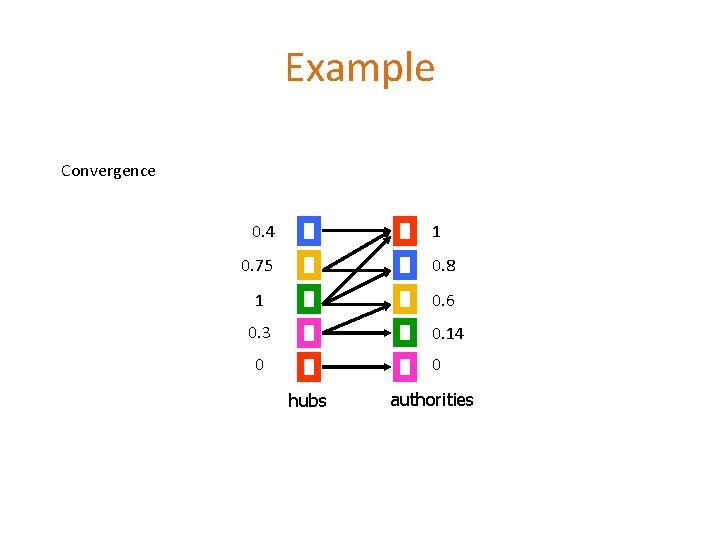
Example Convergence 0. 4 1 0. 75 0. 8 1 0. 6 0. 3 0. 14 0 0 hubs authorities

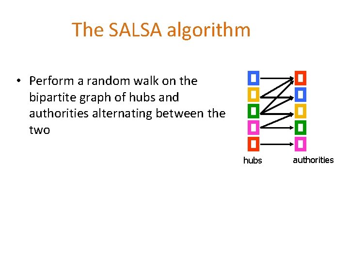
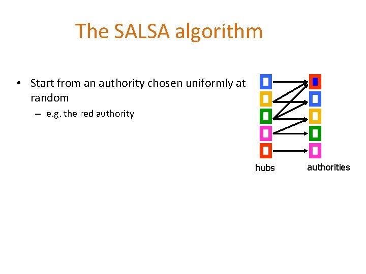
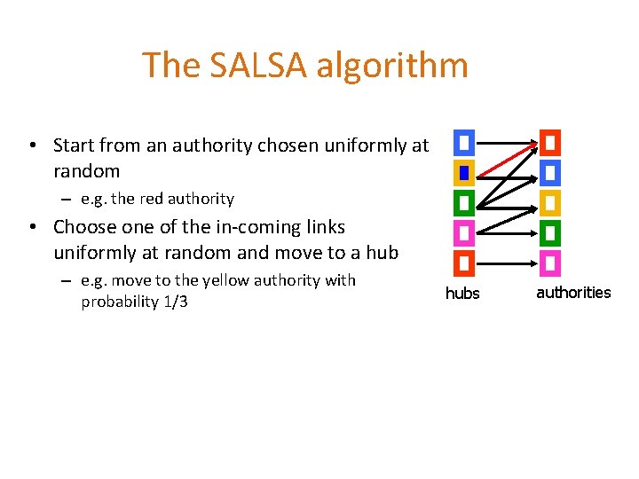
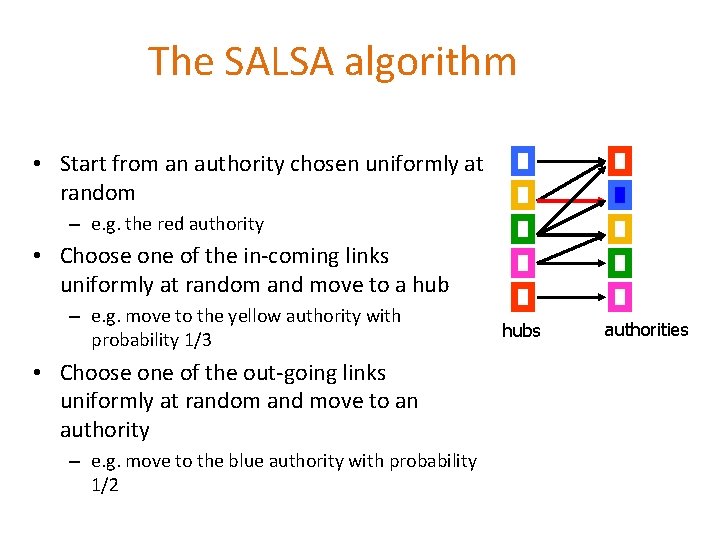
The SALSA algorithm • Perform a random walk on the bipartite graph of hubs and authorities alternating between the two hubs authorities

The SALSA algorithm • Start from an authority chosen uniformly at random – e. g. the red authority hubs authorities

The SALSA algorithm • Start from an authority chosen uniformly at random – e. g. the red authority • Choose one of the in-coming links uniformly at random and move to a hub – e. g. move to the yellow authority with probability 1/3 hubs authorities

The SALSA algorithm • Start from an authority chosen uniformly at random – e. g. the red authority • Choose one of the in-coming links uniformly at random and move to a hub – e. g. move to the yellow authority with probability 1/3 • Choose one of the out-going links uniformly at random and move to an authority – e. g. move to the blue authority with probability 1/2 hubs authorities

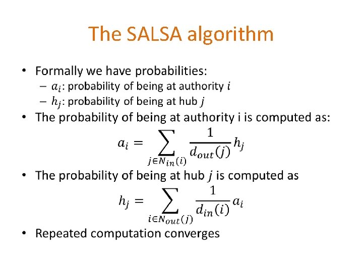
The SALSA algorithm •

The SALSA algorithm [LM 00] • hubs authorities

ABSORBING RANDOM WALKS LABEL PROPAGATION OPINION FORMATION ON SOCIAL NETWORKS

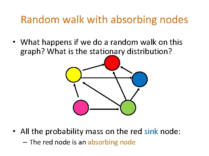
Random walk with absorbing nodes • What happens if we do a random walk on this graph? What is the stationary distribution? • All the probability mass on the red sink node: – The red node is an absorbing node

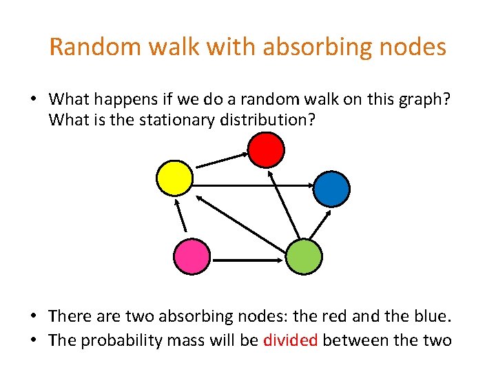
Random walk with absorbing nodes • What happens if we do a random walk on this graph? What is the stationary distribution? • There are two absorbing nodes: the red and the blue. • The probability mass will be divided between the two

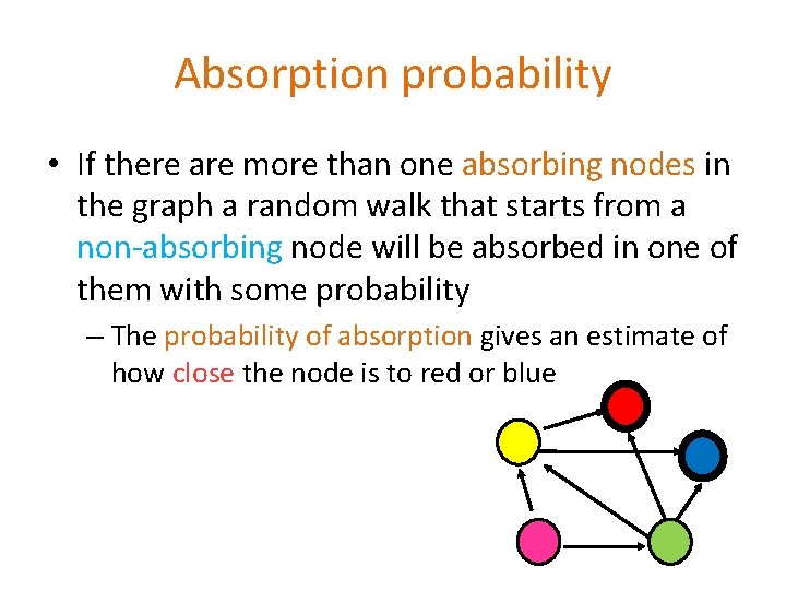
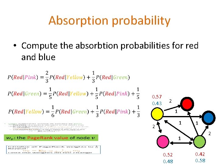
Absorption probability • If there are more than one absorbing nodes in the graph a random walk that starts from a non-absorbing node will be absorbed in one of them with some probability – The probability of absorption gives an estimate of how close the node is to red or blue

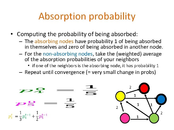
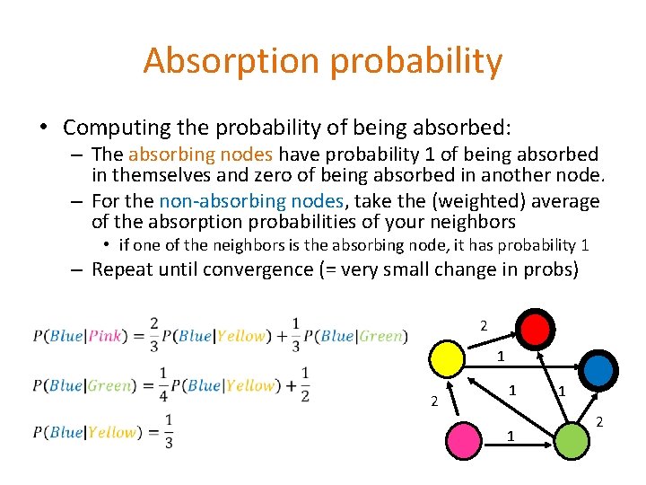
Absorption probability • Computing the probability of being absorbed: – The absorbing nodes have probability 1 of being absorbed in themselves and zero of being absorbed in another node. – For the non-absorbing nodes, take the (weighted) average of the absorption probabilities of your neighbors • if one of the neighbors is the absorbing node, it has probability 1 – Repeat until convergence (= very small change in probs) 2 1 1 1 2

Absorption probability • Computing the probability of being absorbed: – The absorbing nodes have probability 1 of being absorbed in themselves and zero of being absorbed in another node. – For the non-absorbing nodes, take the (weighted) average of the absorption probabilities of your neighbors • if one of the neighbors is the absorbing node, it has probability 1 – Repeat until convergence (= very small change in probs) 2 1 1 1 2

Why do we care? • Why do we care to compute the absorbtion probability to sink nodes? • Given a graph (directed or undirected) we can choose to make some nodes absorbing. – Simply direct all edges incident on the chosen nodes towards them. • The absorbing random walk provides a measure of proximity of non-absorbing nodes to the chosen nodes. – Useful for understanding proximity in graphs – Useful for propagation in the graph • E. g, on a social network some nodes have high income, some have low income, to which income class is a non-absorbing node closer?

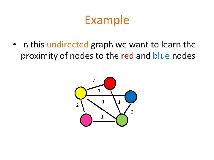
Example • In this undirected graph we want to learn the proximity of nodes to the red and blue nodes 2 1 1 1 2

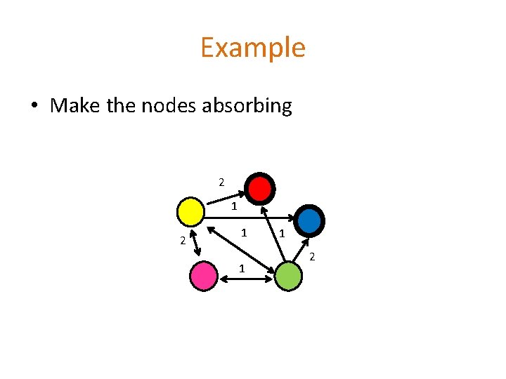
Example • Make the nodes absorbing 2 1 1 1 2

Absorption probability • Compute the absorbtion probabilities for red and blue 0. 57 0. 43 2 1 1 2 1 0. 52 0. 48 0. 42 0. 58

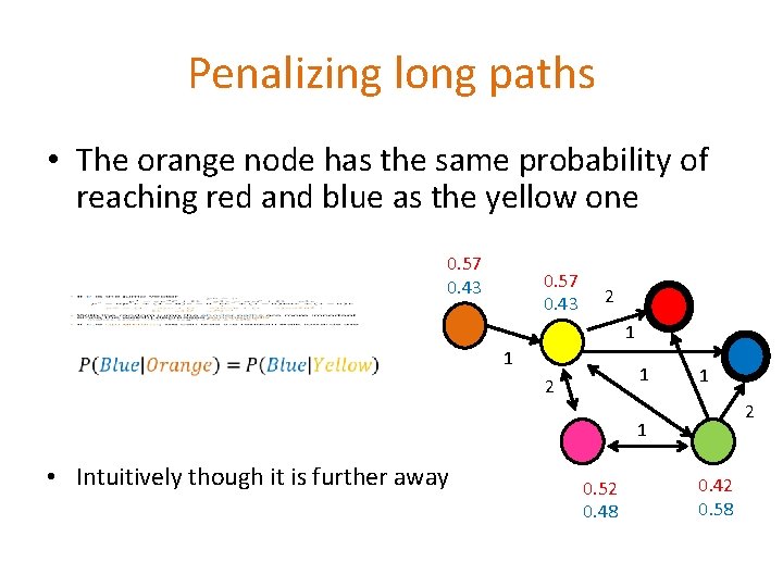
Penalizing long paths • The orange node has the same probability of reaching red and blue as the yellow one 0. 57 0. 43 2 1 1 1 2 1 • Intuitively though it is further away 0. 52 0. 48 0. 42 0. 58

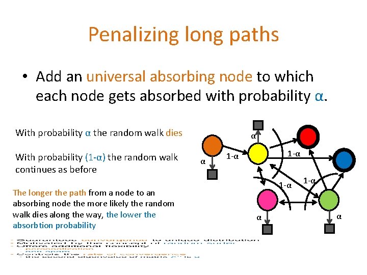
Penalizing long paths • Add an universal absorbing node to which each node gets absorbed with probability α. With probability α the random walk dies With probability (1 -α) the random walk continues as before The longer the path from a node to an absorbing node the more likely the random walk dies along the way, the lower the absorbtion probability α α 1 -α 1 -α α

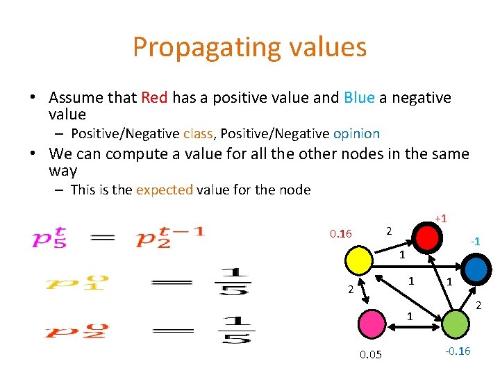
Propagating values • Assume that Red has a positive value and Blue a negative value – Positive/Negative class, Positive/Negative opinion • We can compute a value for all the other nodes in the same way – This is the expected value for the node +1 2 0. 16 -1 1 1 2 1 0. 05 -0. 16

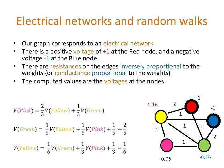
Electrical networks and random walks • Our graph corresponds to an electrical network • There is a positive voltage of +1 at the Red node, and a negative voltage -1 at the Blue node • There are resistances on the edges inversely proportional to the weights (or conductance proportional to the weights) • The computed values are the voltages at the nodes +1 2 0. 16 -1 1 1 2 1 0. 05 -0. 16

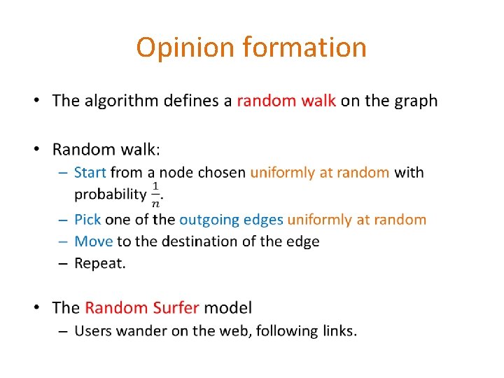
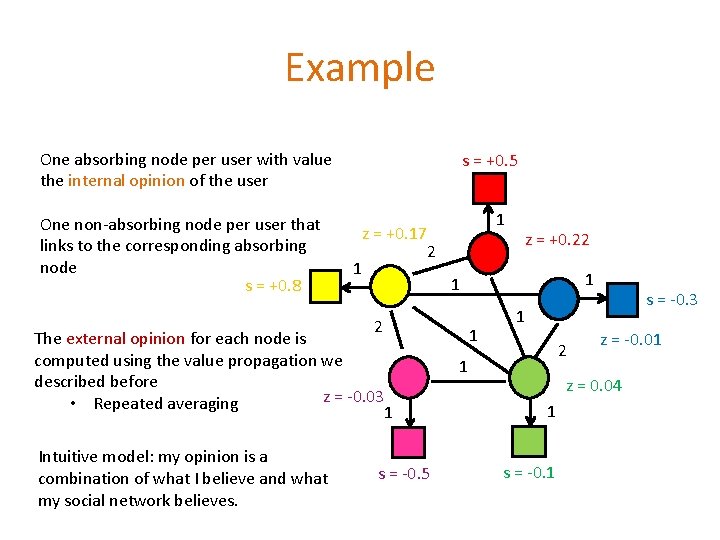
Opinion formation •

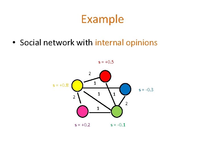
Example • Social network with internal opinions s = +0. 5 2 1 s = +0. 8 2 1 1 s = +0. 2 s = -0. 3 1 2 s = -0. 1

Example One absorbing node per user with value the internal opinion of the user One non-absorbing node per user that links to the corresponding absorbing node s = +0. 8 s = +0. 5 z = +0. 17 2 1 1 Intuitive model: my opinion is a combination of what I believe and what my social network believes. s = -0. 5 1 1 2 The external opinion for each node is computed using the value propagation we described before z = -0. 03 • Repeated averaging 1 z = +0. 22 1 s = -0. 3 1 2 1 z = -0. 01 z = 0. 04 1 s = -0. 1

Transductive learning • If we have a graph of relationships and some labels on some nodes we can propagate them to the remaining nodes – Make the labeled nodes to be absorbing and compute the probability for the rest of the graph – E. g. , a social network where some people are tagged as spammers – E. g. , the movie-actor graph where some movies are tagged as action or comedy. • This is a form of semi-supervised learning – We make use of the unlabeled data, and the relationships • It is also called transductive learning because it does not produce a model, but just labels the unlabeled data that is at hand. – Contrast to inductive learning that learns a model and can label any new example

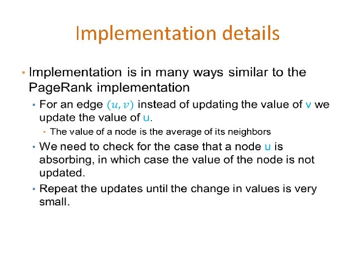
Implementation details •