Social Networks and Social Media 342021 Social Media

Social Networks and Social Media 3/4/2021

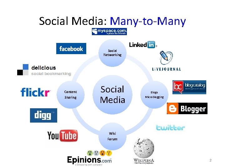
Social Media: Many-to-Many Social Networking Content Sharing Social Media Blogs Microblogging Wiki Forum 2

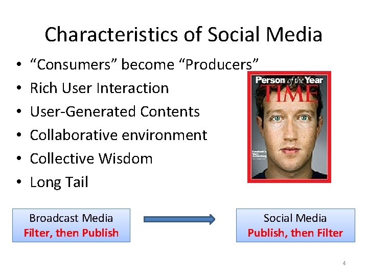
Characteristics of Social Media • • • “Consumers” become “Producers” Rich User Interaction User-Generated Contents Collaborative environment Collective Wisdom Long Tail Broadcast Media Filter, then Publish Social Media Publish, then Filter 4

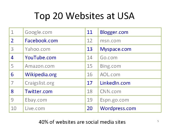
Top 20 Websites at USA 1 2 3 4 Google. com Facebook. com Yahoo. com You. Tube. com 11 12 13 14 Blogger. com msn. com Myspace. com Go. com 5 6 7 8 9 10 Amazon. com Wikipedia. org Craigslist. org Twitter. com Ebay. com Live. com 15 16 17 18 19 20 Bing. com AOL. com Linked. In. com CNN. com Espn. go. com Wordpress. com 40% of websites are social media sites 5

What is Social Network and Social Media • Social Network – The networks formed by individuals • Social Media – social network + media • media = content of twitter, tag, videos, photos. .

Statistical Properties of Social Networks 3/4/2021

Why do statistics • To understand the networks – Understand their topology and measure their properties – Study their evolution and dynamics – Create realistic models – Create algorithms that make use of the network structure 3/4/2021

Interesting Questions: demonstration • Some interesting questions – What do social networks look like, on a large scale? – How do networks behave over time? – How do the non-giant weakly connected components behave over time? – What distributions and patterns do weighted graphs maintain? 3/4/2021

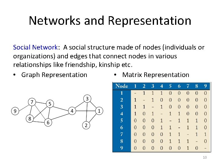
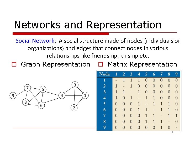
Networks and Representation Social Network: A social structure made of nodes (individuals or organizations) and edges that connect nodes in various relationships like friendship, kinship etc. • Matrix Representation • Graph Representation 10

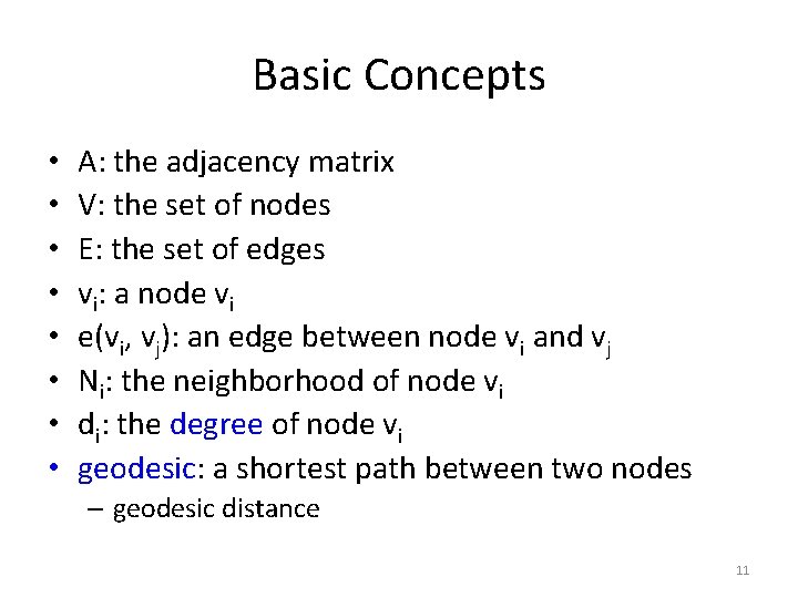
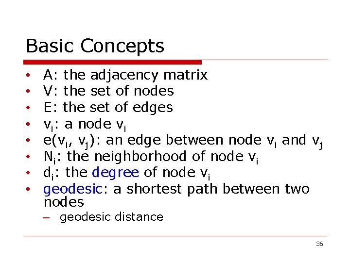
Basic Concepts • • A: the adjacency matrix V: the set of nodes E: the set of edges vi: a node vi e(vi, vj): an edge between node vi and vj Ni: the neighborhood of node vi di: the degree of node vi geodesic: a shortest path between two nodes – geodesic distance 11

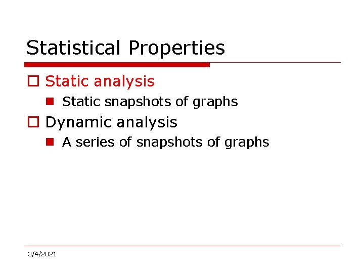
Statistical Properties • Static analysis – Static snapshots of graphs • Dynamic analysis – A series of snapshots of graphs 3/4/2021

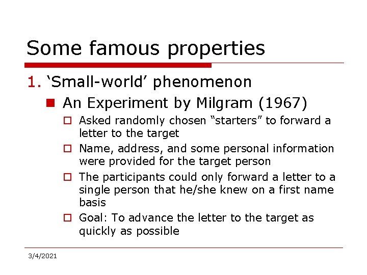
Some famous properties 1. ‘Small-world’ phenomenon – An Experiment by Milgram (1967) • Asked randomly chosen “starters” to forward a letter to the target • Name, address, and some personal information were provided for the target person • The participants could only forward a letter to a single person that he/she knew on a first name basis • Goal: To advance the letter to the target as quickly as possible 3/4/2021

The Milgram Experiment (Wikipedia) Detailed procedure 1. Milgram typically chose individuals in the U. S. cities of Omaha, Nebraska and Wichita, Kansas to be the starting points and Boston, Massachusetts to be the end point of a chain of correspondence – because they were thought to represent a great distance in the United States, both socially and geographically. 2. Information packets were initially sent to "randomly" selected individuals in Omaha or Wichita. They included letters, which detailed the study's purpose, and basic information about a target contact person in Boston. – It additionally contained a roster on which they could write their own name, as well as business reply cards that were pre-addressed to Harvard. 14

The Milgram Experiment (cont. ) 3. Upon receiving the invitation to participate, the recipient was asked whether he or she personally knew the contact person described in the letter. – 4. If so, the person was to forward the letter directly to that person. For the purposes of this study, knowing someone "personally" was defined as knowing them on a first-name basis. In the more likely case that the person did not personally know the target, then the person was to think of a friend or relative they know personally that is more likely to know the target. – A postcard was also mailed to the researchers at Harvard so that they could track the chain's progression toward the target. 15

The Milgram Experiment 5. When and if the package eventually reached the contact person in Boston, the researchers could examine the roster to count the number of times it had been forwarded from person to person. – 3/4/2021 Additionally, for packages that never reached the destination, the incoming postcards helped identify the break point in the chain.

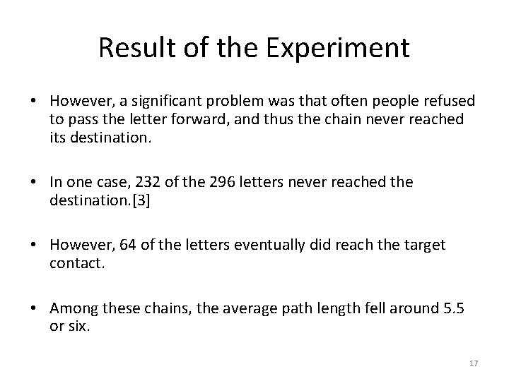
Result of the Experiment • However, a significant problem was that often people refused to pass the letter forward, and thus the chain never reached its destination. • In one case, 232 of the 296 letters never reached the destination. [3] • However, 64 of the letters eventually did reach the target contact. • Among these chains, the average path length fell around 5. 5 or six. 17

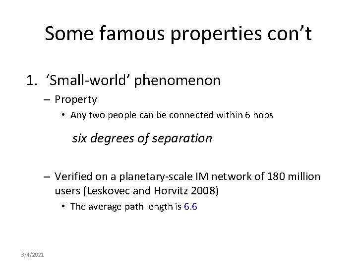
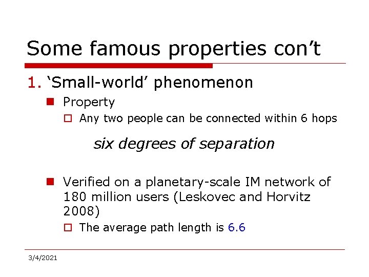
Some famous properties con’t 1. ‘Small-world’ phenomenon – Property • Any two people can be connected within 6 hops six degrees of separation – Verified on a planetary-scale IM network of 180 million users (Leskovec and Horvitz 2008) • The average path length is 6. 6 3/4/2021

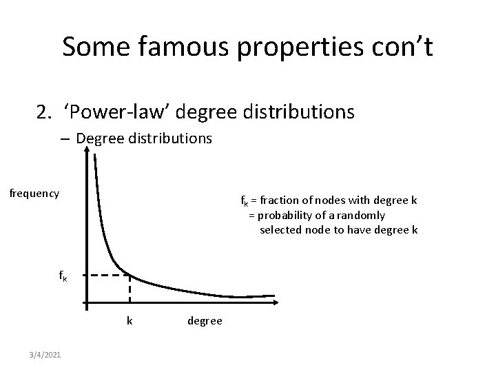
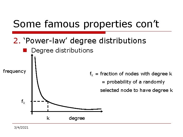
Some famous properties con’t 2. ‘Power-law’ degree distributions – Degree distributions frequency fk = fraction of nodes with degree k = probability of a randomly selected node to have degree k fk k 3/4/2021 degree

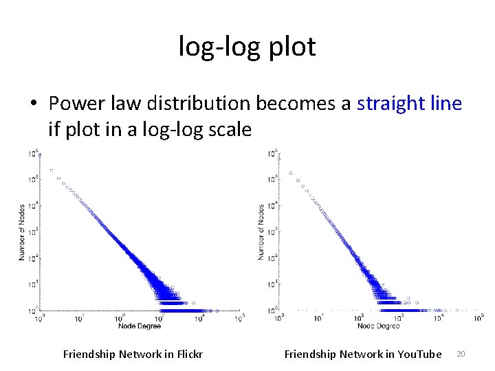
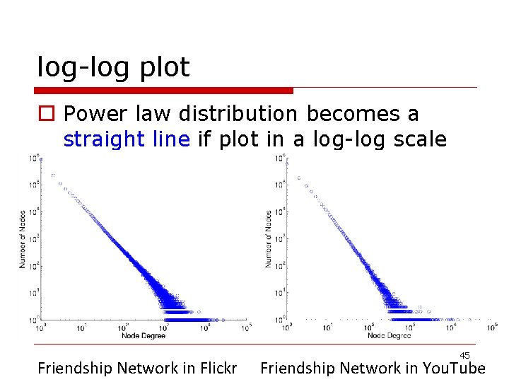
log-log plot • Power law distribution becomes a straight line if plot in a log-log scale Friendship Network in Flickr Friendship Network in You. Tube 20

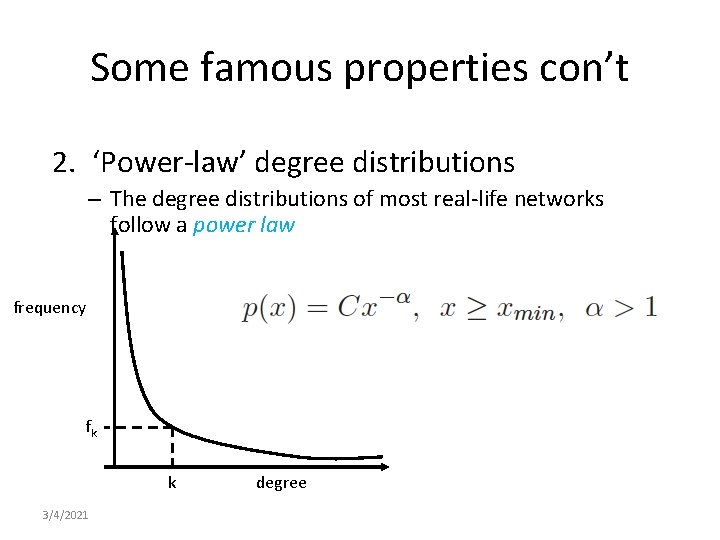
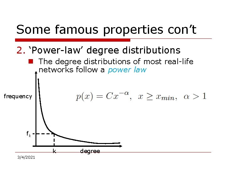
Some famous properties con’t 2. ‘Power-law’ degree distributions – The degree distributions of most real-life networks follow a power law frequency fk k 3/4/2021 degree

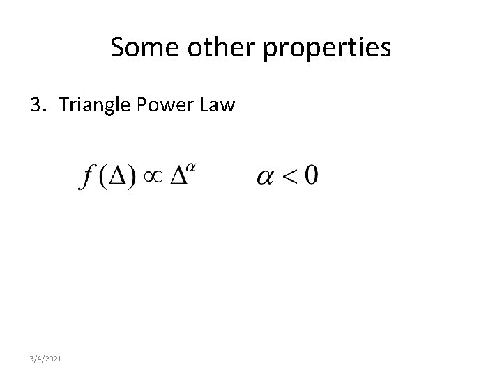
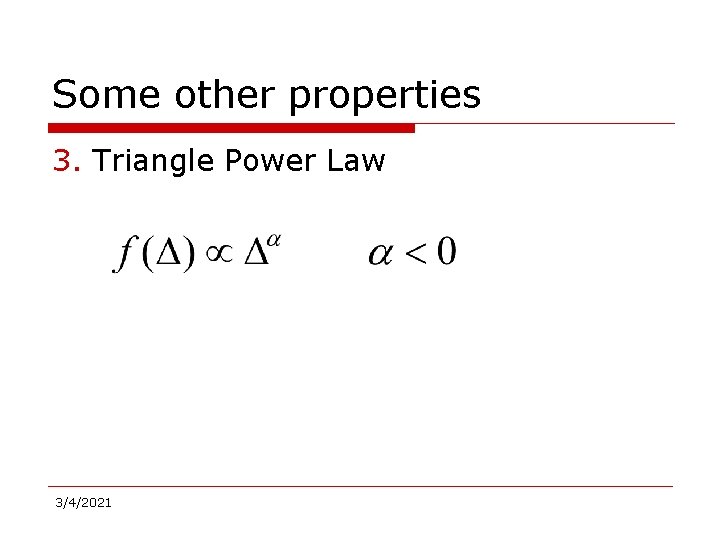
Some other properties 3. Triangle Power Law 3/4/2021

Some other properties 4. Eigenvalue Power Law l The 20 or so largest eigenvalues of the adjacency matrix are power law distributed l This is consequence of the “Degree Power Law” 3/4/2021

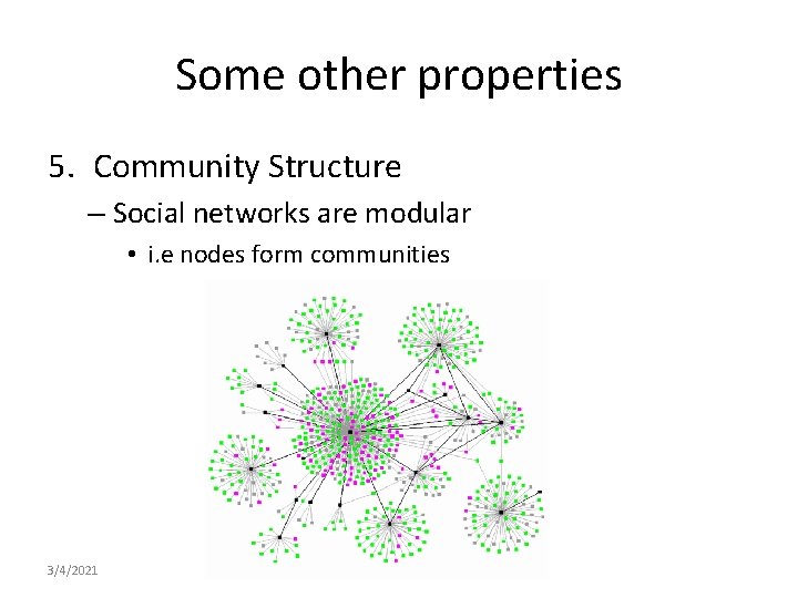
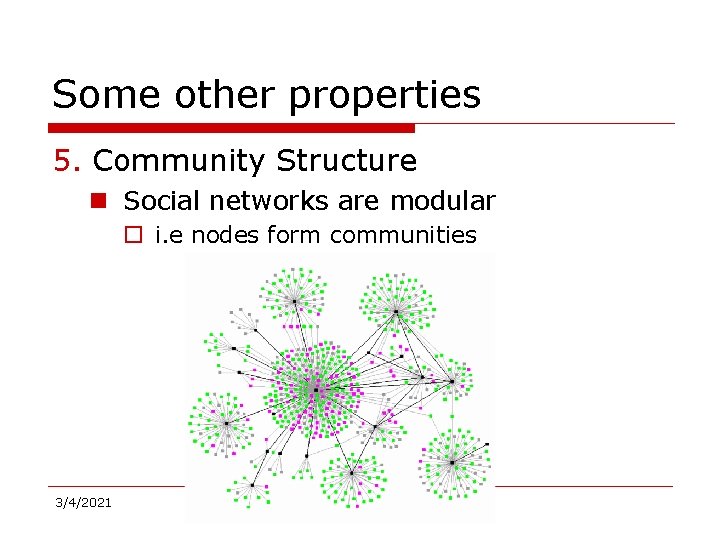
Some other properties 5. Community Structure – Social networks are modular • i. e nodes form communities 3/4/2021

Statistical Properties • Static analysis – Static snapshots of graphs • Dynamic analysis – A series of snapshots of graphs 3/4/2021

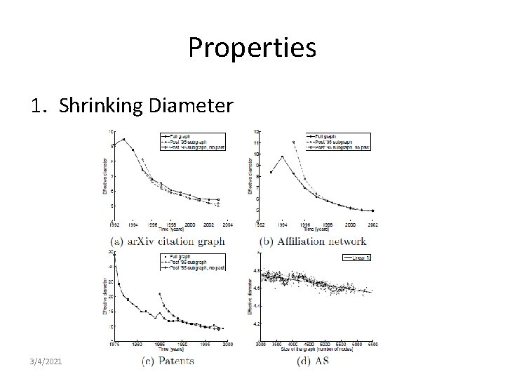
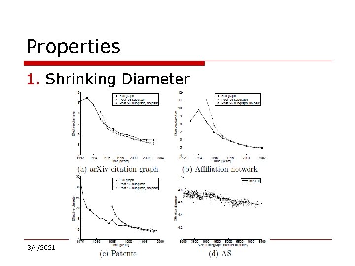
Properties 1. Shrinking Diameter 3/4/2021

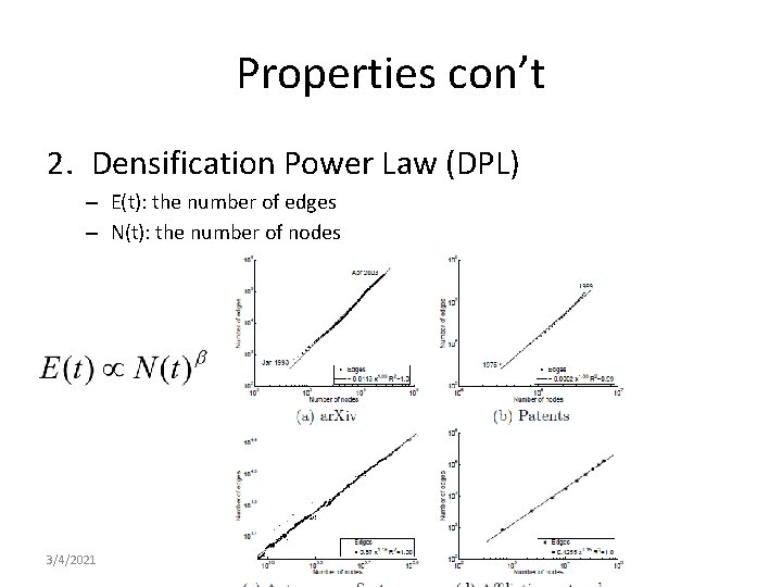
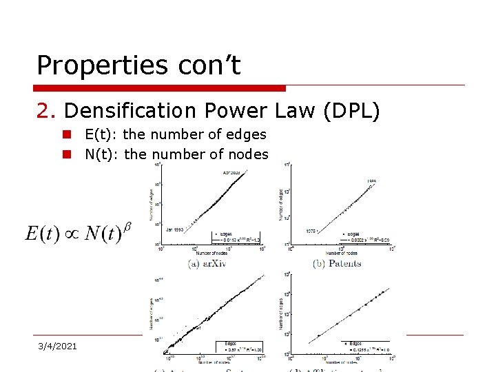
Properties con’t 2. Densification Power Law (DPL) – E(t): the number of edges – N(t): the number of nodes 3/4/2021

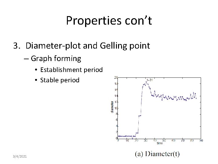
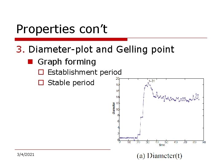
Properties con’t 3. Diameter-plot and Gelling point – Graph forming • Establishment period • Stable period 3/4/2021

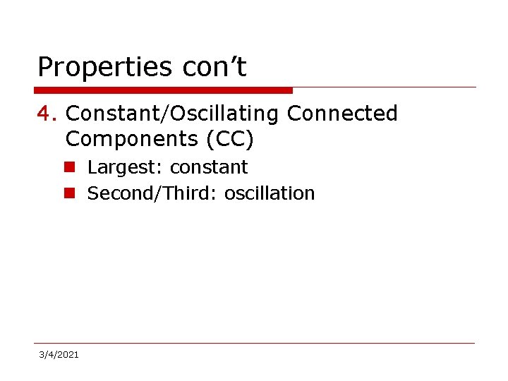
Properties con’t 4. Constant/Oscillating Connected Components (CC) – Largest: constant – Second/Third: oscillation 3/4/2021

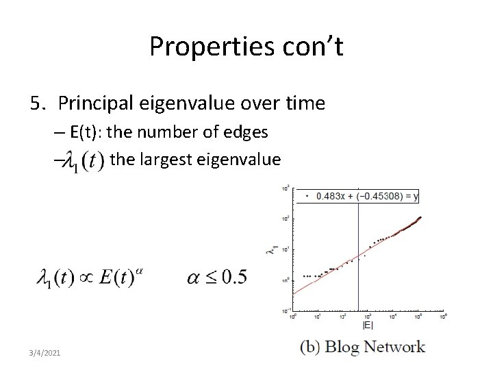
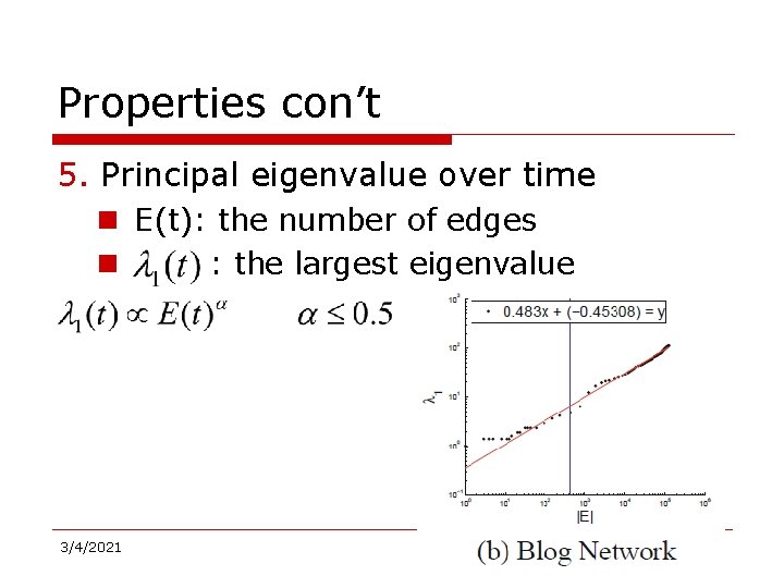
Properties con’t 5. Principal eigenvalue over time – E(t): the number of edges – : the largest eigenvalue 3/4/2021

Conclusion • Usefulness of the statistical properties – Understanding human behaviors – Anomalous graphs/subgraphs detection – Identifying authorities and search algorithms – Prepare resources based on the prediction –… 3/4/2021

Statistical Properties of Social Networks 3/4/2021

Why do statistics o To understand the networks n Understand their topology and measure their properties n Study their evolution and dynamics n Create realistic models n Create algorithms that make use of the network structure 3/4/2021

Interesting Questions: demonstration o Some interesting questions n What do social networks look like, on a large scale? n How do networks behave over time? n How do the non-giant weakly connected components behave over time? n What distributions and patterns do weighted graphs maintain? 3/4/2021

Networks and Representation Social Network: A social structure made of nodes (individuals or organizations) and edges that connect nodes in various relationships like friendship, kinship etc. o Graph Representation o Matrix Representation 35

Basic Concepts • • A: the adjacency matrix V: the set of nodes E: the set of edges vi: a node vi e(vi, vj): an edge between node vi and vj Ni: the neighborhood of node vi di: the degree of node vi geodesic: a shortest path between two nodes – geodesic distance 36

Statistical Properties o Static analysis n Static snapshots of graphs o Dynamic analysis n A series of snapshots of graphs 3/4/2021

Some famous properties 1. ‘Small-world’ phenomenon n An Experiment by Milgram (1967) o Asked randomly chosen “starters” to forward a letter to the target o Name, address, and some personal information were provided for the target person o The participants could only forward a letter to a single person that he/she knew on a first name basis o Goal: To advance the letter to the target as quickly as possible 3/4/2021

The Milgram Experiment (Wikipedia) Detailed procedure 1. Milgram typically chose individuals in the U. S. cities of Omaha, Nebraska and Wichita, Kansas to be the starting points and Boston, Massachusetts to be the end point of a chain of correspondence n because they were thought to represent a great distance in the United States, both socially and geographically. 2. Information packets were initially sent to "randomly" selected individuals in Omaha or Wichita. They included letters, which detailed the study's purpose, and basic information about a target contact person in Boston. n It additionally contained a roster on which they could write their own name, as well as business reply cards that were pre-addressed to Harvard. 39

The Milgram Experiment (cont. ) 3. Upon receiving the invitation to participate, the recipient was asked whether he or she personally knew the contact person described in the letter. n If so, the person was to forward the letter directly to that person. For the purposes of this study, knowing someone "personally" was defined as knowing them on a first-name basis. 4. In the more likely case that the person did not personally know the target, then the person was to think of a friend or relative they know personally that is more likely to know the target. n A postcard was also mailed to the researchers at Harvard so that they could track the chain's progression toward the target. 40

The Milgram Experiment 5. When and if the package eventually reached the contact person in Boston, the researchers could examine the roster to count the number of times it had been forwarded from person to person. n 3/4/2021 Additionally, for packages that never reached the destination, the incoming postcards helped identify the break point in the chain.

Result of the Experiment • However, a significant problem was that often people refused to pass the letter forward, and thus the chain never reached its destination. • In one case, 232 of the 296 letters never reached the destination. [3] • However, 64 of the letters eventually did reach the target contact. • Among these chains, the average path length fell around 5. 5 or six. 42

Some famous properties con’t 1. ‘Small-world’ phenomenon n Property o Any two people can be connected within 6 hops six degrees of separation n Verified on a planetary-scale IM network of 180 million users (Leskovec and Horvitz 2008) o The average path length is 6. 6 3/4/2021

Some famous properties con’t 2. ‘Power-law’ degree distributions n Degree distributions frequency fk = fraction of nodes with degree k = probability of a randomly selected node to have degree k fk k 3/4/2021 degree

log-log plot o Power law distribution becomes a straight line if plot in a log-log scale Friendship Network in Flickr 45 Friendship Network in You. Tube

Some famous properties con’t 2. ‘Power-law’ degree distributions n The degree distributions of most real-life networks follow a power law frequency fk k 3/4/2021 degree

Some other properties 3. Triangle Power Law 3/4/2021

Some other properties 4. Eigenvalue Power Law l The 20 or so largest eigenvalues of the adjacency matrix are power law distributed l This is consequence of the “Degree Power Law” 3/4/2021

Some other properties 5. Community Structure n Social networks are modular o i. e nodes form communities 3/4/2021

Statistical Properties o Static analysis n Static snapshots of graphs o Dynamic analysis n A series of snapshots of graphs 3/4/2021

Properties 1. Shrinking Diameter 3/4/2021

Properties con’t 2. Densification Power Law (DPL) n E(t): the number of edges n N(t): the number of nodes 3/4/2021

Properties con’t 3. Diameter-plot and Gelling point n Graph forming o Establishment period o Stable period 3/4/2021

Properties con’t 4. Constant/Oscillating Connected Components (CC) n Largest: constant n Second/Third: oscillation 3/4/2021

Properties con’t 5. Principal eigenvalue over time n E(t): the number of edges n : the largest eigenvalue 3/4/2021

Conclusion o Usefulness of the statistical properties n Understanding human behaviors n Anomalous graphs/subgraphs detection n Identifying authorities and search algorithms n Prepare resources based on the prediction n … 3/4/2021

Community Discovery in Social Networks 3/4/2021

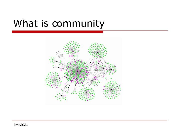
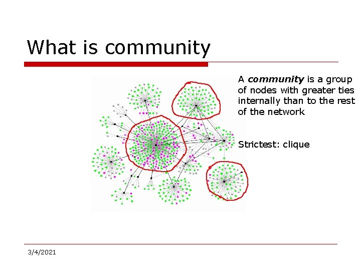
What is community 3/4/2021

What is community A community is a group of nodes with greater ties internally than to the rest of the network Strictest: clique 3/4/2021

Why community exists? o Why communities in social media? n Human beings are social n Easy-to-use social media allows people to extend their social life in unprecedented ways n Difficult to meet friends in the physical world, but much easier to find friend online with similar interests n Interactions between nodes can help determine communities 3/4/2021

Why do community discovery o Why? n Understand underpin social structure and its evolution n Study the social behavior of human/animals n Set proxy caches n Detect link farms n Do personalized recommendation n Enable efficient message routing and posting in mobile ad-hoc networks n Enable efficient customer feedback n … 3/4/2021

Discovering Algorithms o Outline n Overview n Quality Estimation n Some Algorithms 3/4/2021

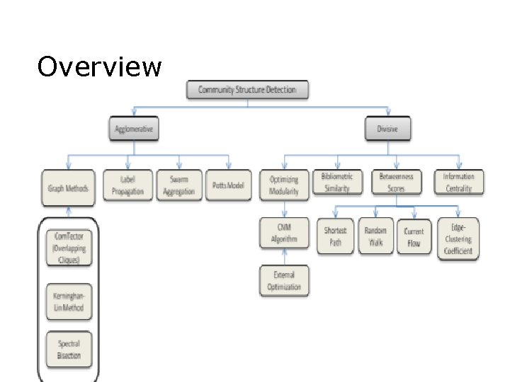
Overview 3/4/2021

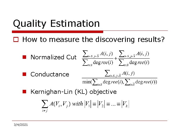
Quality Estimation o How to measure the discovering results? n Normalized Cut n Conductance n Kernighan-Lin (KL) objective 3/4/2021

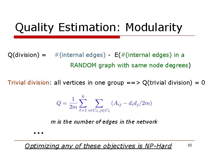
Quality Estimation: Modularity Q(division) = #(internal edges) - E(#(internal edges) in a RANDOM graph with same node degrees) Trivial division: all vertices in one group ==> Q(trivial division) = 0 … m is the number of edges in the network Optimizing any of these objectives is NP-Hard 65

Discovering Algorithms o Outline n Overview n Quality Estimation n Some Algorithms 3/4/2021

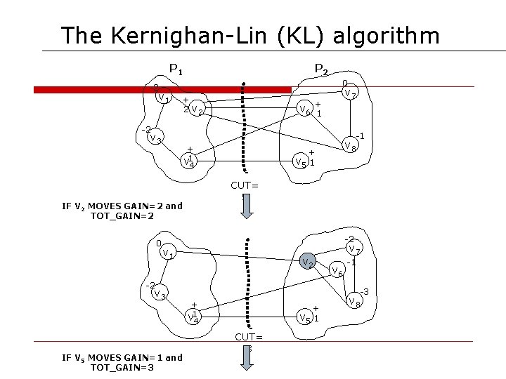
The Kernighan-Lin (KL) algorithm P 1 P 2 0 -2 v 1 + 2 v 7 + v 6 1 -2 v 3 -1 + v 1 4 CUT= 5 IF V 2 MOVES GAIN=2 and TOT_GAIN=2 0 v 8 + v 5 1 -2 v 1 v 2 -2 v 3 v 6 -1 -3 + v 1 + v 5 1 4 IF V 5 MOVES GAIN=1 and TOT_GAIN=3 v 7 CUT= 3 v 8

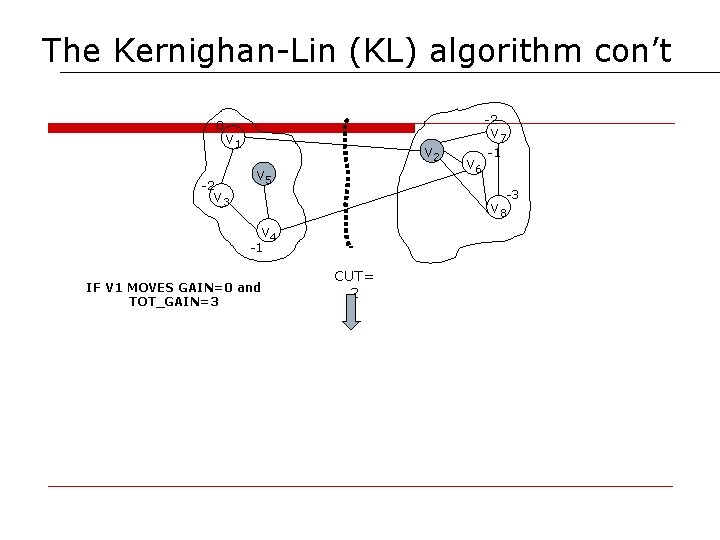
The Kernighan-Lin (KL) algorithm con’t 0 -2 -2 v 1 v 3 v 2 v 5 v 7 v 6 -1 -3 v 8 v 4 -1 IF V 1 MOVES GAIN=0 and TOT_GAIN=3 CUT= 2

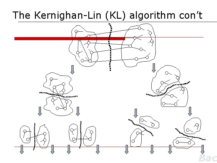
The Kernighan-Lin (KL) algorithm con’t Bac

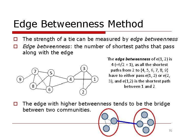
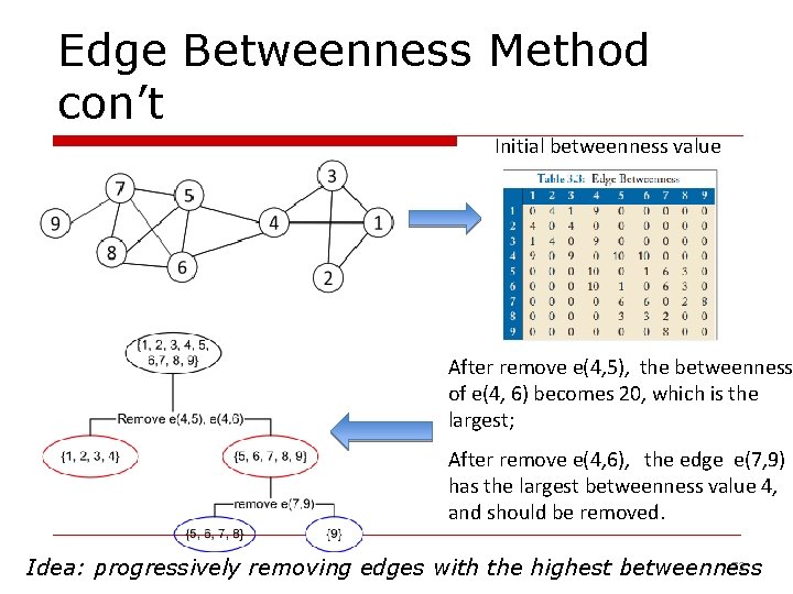
Edge Betweenness Method o The strength of a tie can be measured by edge betweenness o Edge betweenness: the number of shortest paths that pass along with the edge The edge betweenness of e(1, 2) is 4 (=6/2 + 1), as all the shortest paths from 2 to {4, 5, 6, 7, 8, 9} have to either pass e(1, 2) or e(2, 3), and e(1, 2) is the shortest path between 1 and 2 o The edge with higher betweenness tends to be the bridge between two communities. 70

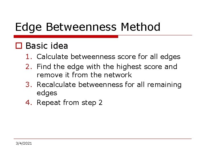
Edge Betweenness Method o Basic idea 1. Calculate betweenness score for all edges 2. Find the edge with the highest score and remove it from the network 3. Recalculate betweenness for all remaining edges 4. Repeat from step 2 3/4/2021

Edge Betweenness Method con’t Initial betweenness value After remove e(4, 5), the betweenness of e(4, 6) becomes 20, which is the largest; After remove e(4, 6), the edge e(7, 9) has the largest betweenness value 4, and should be removed. 72 Idea: progressively removing edges with the highest betweenness

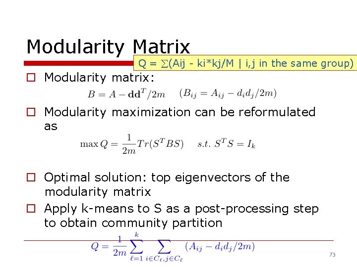
Modularity Matrix Q = (Aij - ki*kj/M | i, j in the same group) o Modularity matrix: o Modularity maximization can be reformulated as o Optimal solution: top eigenvectors of the modularity matrix o Apply k-means to S as a post-processing step to obtain community partition 73

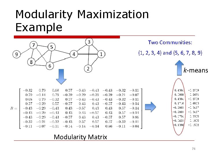
Modularity Maximization Example Two Communities: {1, 2, 3, 4} and {5, 6, 7, 8, 9} k-means Modularity Matrix 74

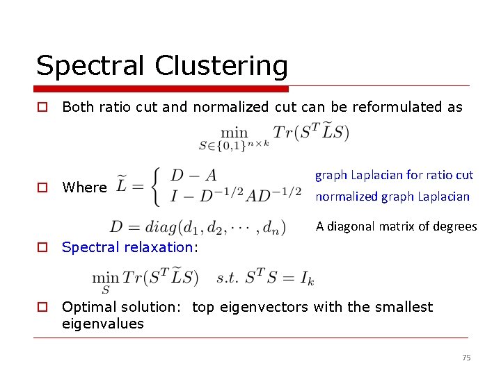
Spectral Clustering o Both ratio cut and normalized cut can be reformulated as o Where graph Laplacian for ratio cut normalized graph Laplacian A diagonal matrix of degrees o Spectral relaxation: o Optimal solution: top eigenvectors with the smallest eigenvalues 75

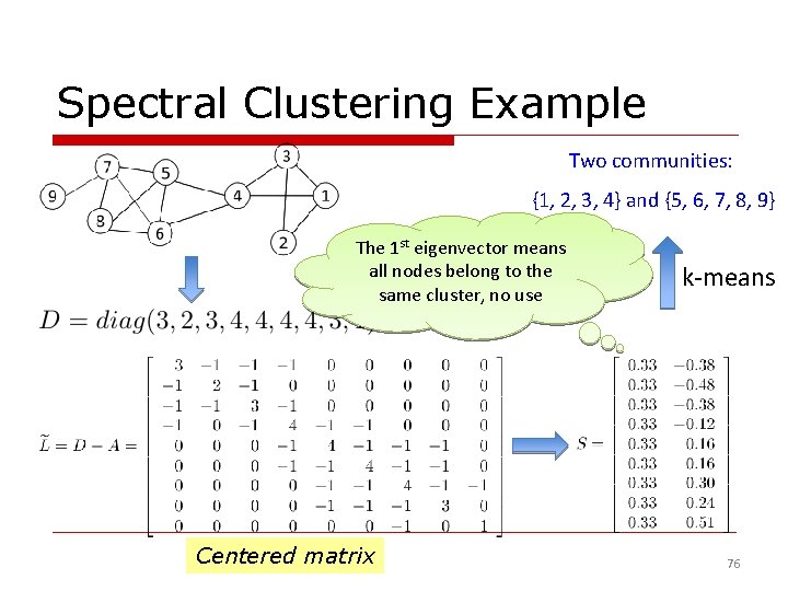
Spectral Clustering Example Two communities: {1, 2, 3, 4} and {5, 6, 7, 8, 9} The 1 st eigenvector means all nodes belong to the same cluster, no use Centered matrix k-means 76

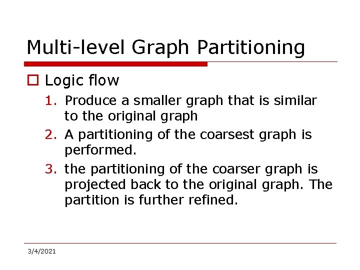
Multi-level Graph Partitioning o Logic flow 1. Produce a smaller graph that is similar to the original graph 2. A partitioning of the coarsest graph is performed. 3. the partitioning of the coarser graph is projected back to the original graph. The partition is further refined. 3/4/2021

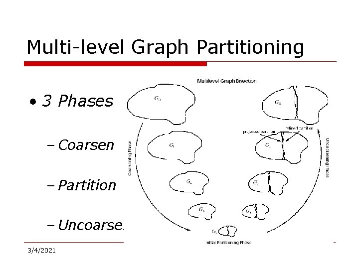
Multi-level Graph Partitioning • 3 Phases – Coarsen – Partition – Uncoarsen 3/4/2021

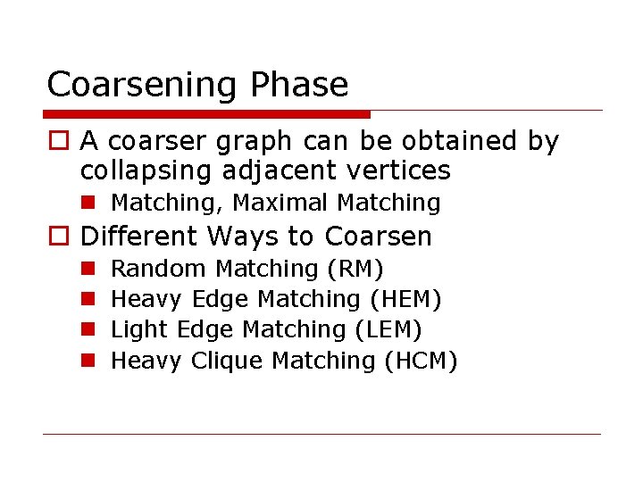
Coarsening Phase o A coarser graph can be obtained by collapsing adjacent vertices n Matching, Maximal Matching o Different Ways to Coarsen n n Random Matching (RM) Heavy Edge Matching (HEM) Light Edge Matching (LEM) Heavy Clique Matching (HCM)

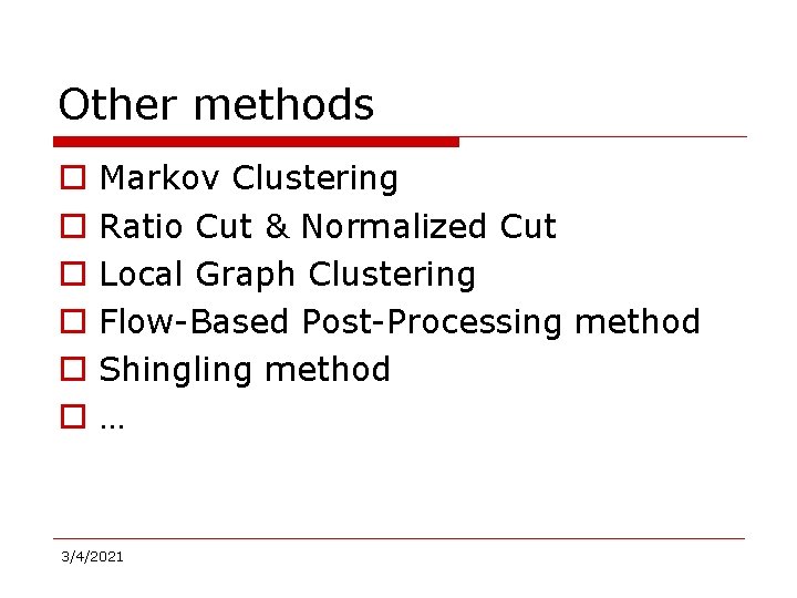
Other methods o o o Markov Clustering Ratio Cut & Normalized Cut Local Graph Clustering Flow-Based Post-Processing method Shingling method … 3/4/2021

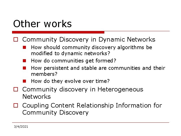
Other works o Community Discovery in Dynamic Networks n How should community discovery algorithms be modified to dynamic networks? n How do communities get formed? n How persistent and stable are communities and their members? n How do they evolve over time? o Community discovery in Heterogeneous Networks o Coupling Content Relationship Information for Community Discovery 3/4/2021

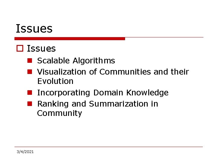
Issues o Issues n Scalable Algorithms n Visualization of Communities and their Evolution n Incorporating Domain Knowledge n Ranking and Summarization in Community 3/4/2021

Reference 1. 2. Chapter 3, Community Detection and Mining in Social Media. Lei Tang and Huan Liu, Morgan & Claypool, September, 2010. http: //www. google. com/url? sa=t&rct=j&q=&esrc=s&source=w eb&cd=1&ved=0 CFYQFj. AA&url=http%3 A%2 F%2 Fdelab. csd. au th. gr%2 Fcourses%2 Fc_mmdb%2 Fmmdb-2011 -2012 metis. ppt&ei=SEIj. UJa 8 OKm 0 i. Qf 0 v. YGIBg&usg=AFQj. CNEP 5 NPt_ GFIpn. TQXye 8 l 3 Fzc 8 EHAg 3/4/2021

Link Prediction in Social Networks 3/4/2021

Outline • Link Prediction Problems – Social Network – Recommender system • Algorithms of Link Prediction – Supervised Methods – Collaborative Filtering • Recommender System and The Netflixprize • References

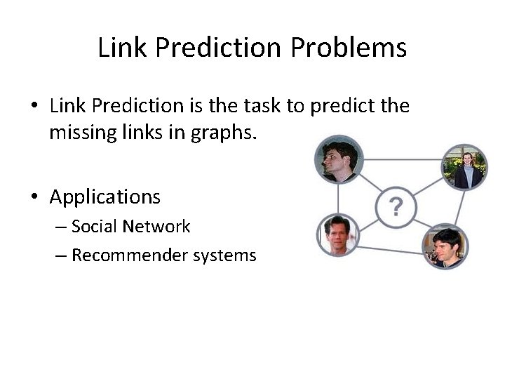
Link Prediction Problems • Link Prediction is the task to predict the missing links in graphs. • Applications – Social Network – Recommender systems

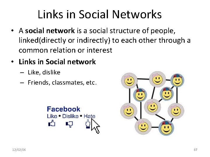
Links in Social Networks • A social network is a social structure of people, linked(directly or indirectly) to each other through a common relation or interest • Links in Social network – Like, dislike – Friends, classmates, etc. 12/02/06 87

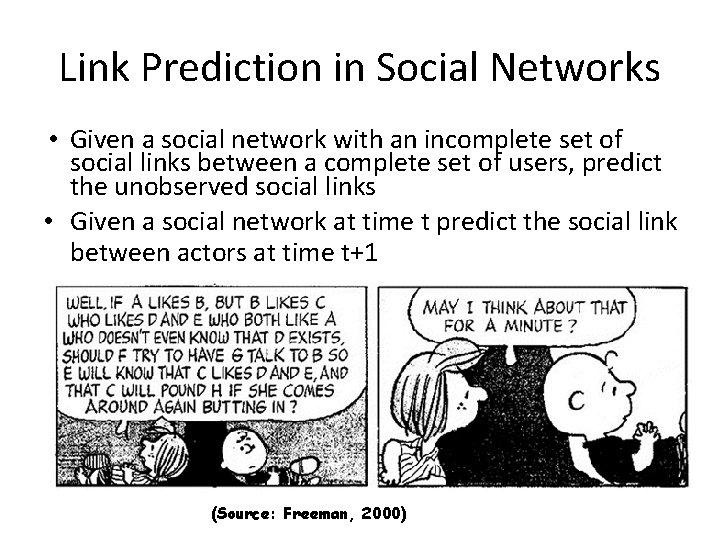
Link Prediction in Social Networks • Given a social network with an incomplete set of social links between a complete set of users, predict the unobserved social links • Given a social network at time t predict the social link between actors at time t+1 (Source: Freeman, 2000)

Link Prediction in Recommender Systems • Recommender Systems

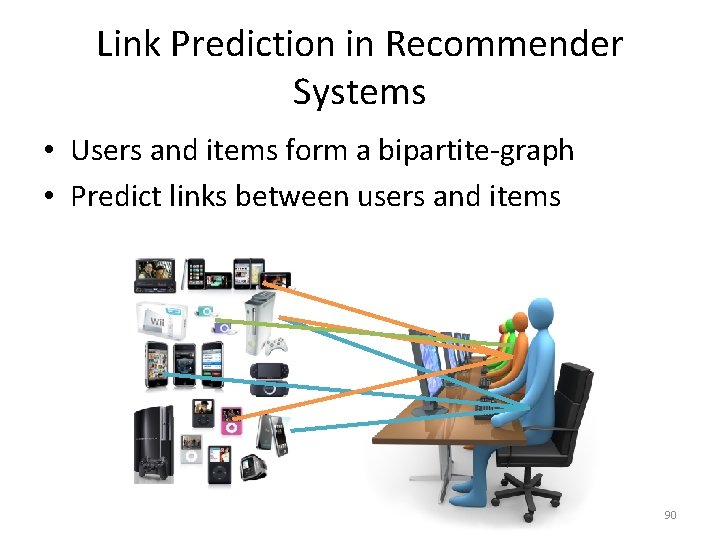
Link Prediction in Recommender Systems • Users and items form a bipartite-graph • Predict links between users and items 90

Predicting Link Existence • Predicting whether a link exists between two items – web: predict whethere will be a link between two pages – cite: predicting whether a paper will cite another paper – epi: predicting who a patient’s contacts are • Predicting whether a link exists between items and users 3/4/2021 91

Everyday Examples of Link Prediction/Collaborative Filtering. . . • • • Search engine Shopping Reading Social. . Common insight: personal tastes are correlated: – If Alice and Bob both like X and Alice likes Y then Bob is more likely to like Y – especially (perhaps) if Bob knows Alice

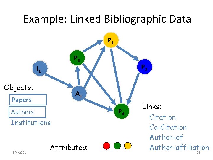
Example: Linked Bibliographic Data P 1 P 3 P 2 I 1 Objects: A 1 Papers Authors P 4 Institutions 3/4/2021 Attributes: Links: Citation Co-Citation Author-of Author-affiliation 93

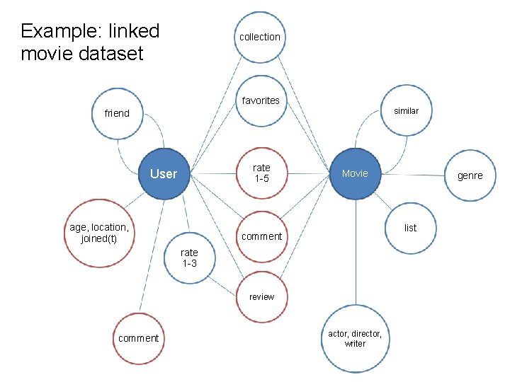
Example: linked movie dataset collection favorites similar friend rate 1 -5 User age, location, joined(t) Movie list comment rate 1 -3 review comment genre actor, director, writer

How to do link prediction? How can you do recommendation based on this item?

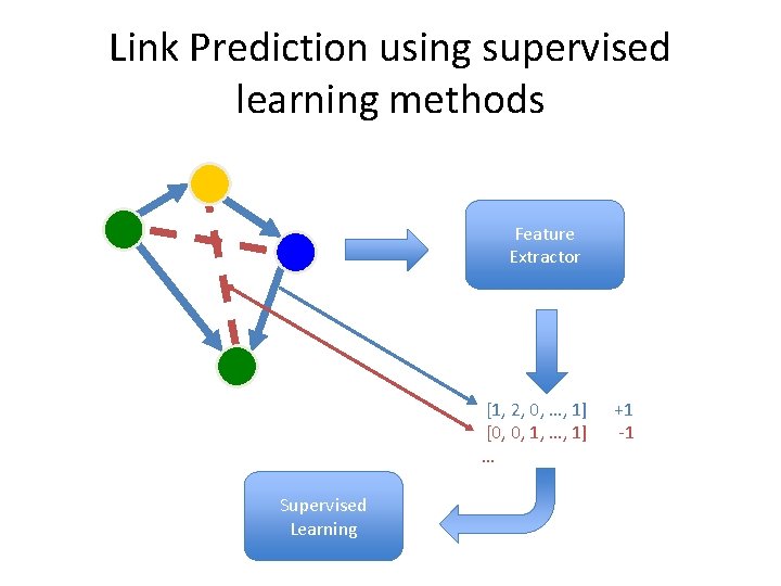
Link Prediction using supervised learning methods P 1 P 3 P 2 Feature Extractor [1, 2, 0, …, 1] +1 [0, 0, 1, …, 1] -1 … Supervised Learning

Supervised Learning Methods [Liben. Nowell and Kleinberg, 2003] • Link prediction as a means to gauge the usefulness of a model • Proximity Features: Common Neighbors, Katz, Jaccard, etc • No single predictor consistently outperforms the others

supervised learning methods [Hasan et al, 2006] • Citation Network (BIOBASE, DBLP) • Use machine learning algorithms to predict future co-authorship (decision tree, k-NN, multilayer perceptron, SVM, RBF network) • Identify a group of features that are most helpful in prediction • Best Predictor Features: Keyword Match count, Sum of neighbors, Sum of Papers, Shortest Distance

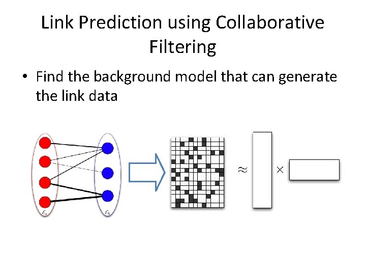
Link Prediction using Collaborative Filtering • Find the background model that can generate the link data

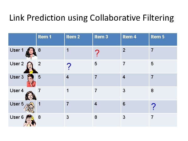
Link Prediction using Collaborative Filtering Item 1 Item 2 Item 3 Item 4 Item 5 User 1 8 1 ? 2 7 User 2 2 ? 5 7 5 User 3 5 4 7 User 4 7 1 7 3 8 User 5 1 7 4 6 ? User 6 8 3 7

Challenges in Link Prediction • Data!!! • Cold Start Problem • Sparsity Problem

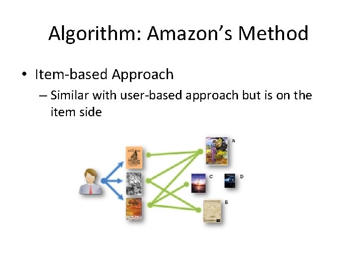
Link Prediction using Collaborative Filtering • Memory-based Approach – User-base approach [Twitter] – item-base approach [Amazon & Youtube] • Model-based Approach – Latent Factor Model [Google News] • Hybrid Approach

Memory-based Approach • Few modeling assumptions • Few tuning parameters to learn • Easy to explain to users – Dear Amazon. com Customer, We've noticed that customers who have purchased or rated How Does the Show Go On: An Introduction to the Theater by Thomas Schumacher have also purchased Princess Protection Program #1: A Royal Makeover (Disney Early Readers). 103

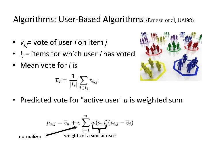
Algorithms: User-Based Algorithms (Breese et al, UAI 98) • vi, j= vote of user i on item j • Ii = items for which user i has voted • Mean vote for i is • Predicted vote for “active user” a is weighted sum normalizer weights of n similar users

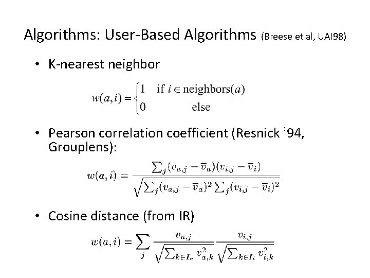
Algorithms: User-Based Algorithms (Breese et al, UAI 98) • K-nearest neighbor • Pearson correlation coefficient (Resnick ’ 94, Grouplens): • Cosine distance (from IR)

Algorithm: Amazon’s Method • Item-based Approach – Similar with user-based approach but is on the item side

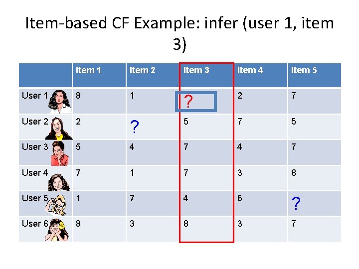
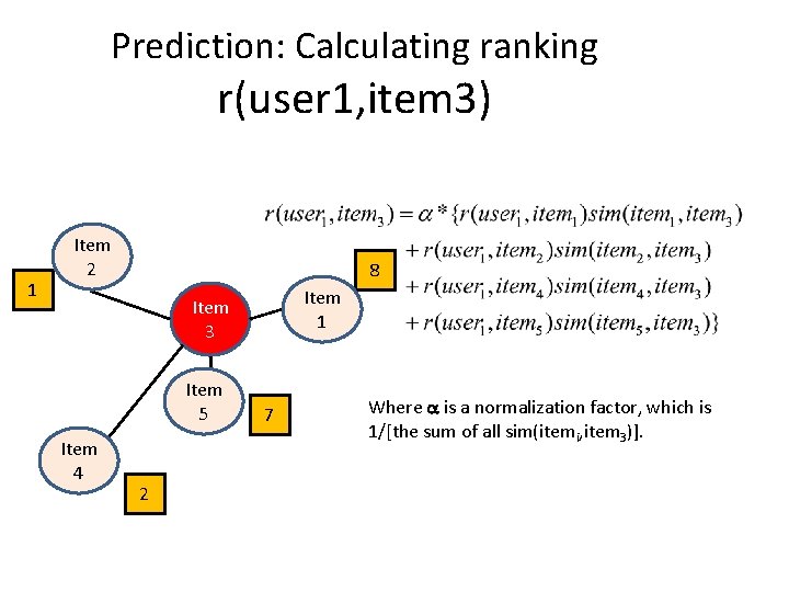
Item-based CF Example: infer (user 1, item 3) Item 1 Item 2 Item 3 Item 4 Item 5 User 1 8 1 ? 2 7 User 2 2 ? 5 7 5 User 3 5 4 7 User 4 7 1 7 3 8 User 5 1 7 4 6 ? User 6 8 3 7

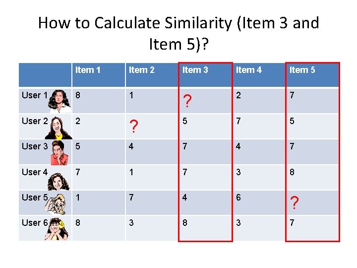
How to Calculate Similarity (Item 3 and Item 5)? Item 1 Item 2 Item 3 Item 4 Item 5 User 1 8 1 ? 2 7 User 2 2 ? 5 7 5 User 3 5 4 7 User 4 7 1 7 3 8 User 5 1 7 4 6 ? User 6 8 3 7

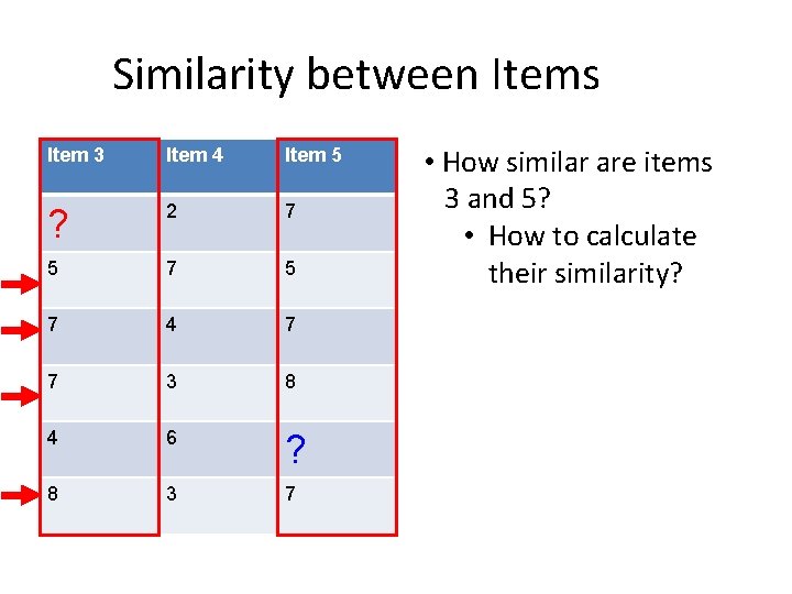
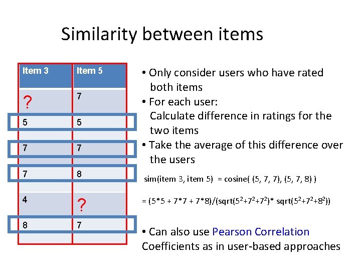
Similarity between Items Item 3 Item 4 Item 5 ? 2 7 5 7 4 7 7 3 8 4 6 ? 8 3 7 • How similar are items 3 and 5? • How to calculate their similarity?

Similarity between items • Only consider users who have rated both items • For each user: Calculate difference in ratings for the two items • Take the average of this difference over the users Item 3 Item 5 ? 7 5 5 7 7 7 8 sim(item 3, item 5) = cosine( (5, 7, 7), (5, 7, 8) ) 4 ? = (5*5 + 7*7 + 7*8)/(sqrt(52+72+72)* sqrt(52+72+82)) 8 7 • Can also use Pearson Correlation Coefficients as in user-based approaches

Prediction: Calculating ranking r(user 1, item 3) 1 Item 2 8 Item 1 Item 3 Item 5 Item 4 2 7 Where a is a normalization factor, which is 1/[the sum of all sim(itemi, item 3)].

Netflixprize

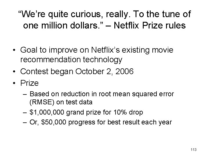
“We’re quite curious, really. To the tune of one million dollars. ” – Netflix Prize rules • Goal to improve on Netflix’s existing movie recommendation technology • Contest began October 2, 2006 • Prize – Based on reduction in root mean squared error (RMSE) on test data – $1, 000 grand prize for 10% drop – Or, $50, 000 progress for best result each year 113

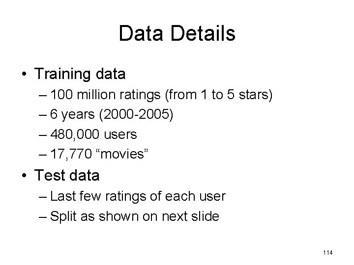
Data Details • Training data – 100 million ratings (from 1 to 5 stars) – 6 years (2000 -2005) – 480, 000 users – 17, 770 “movies” • Test data – Last few ratings of each user – Split as shown on next slide 114

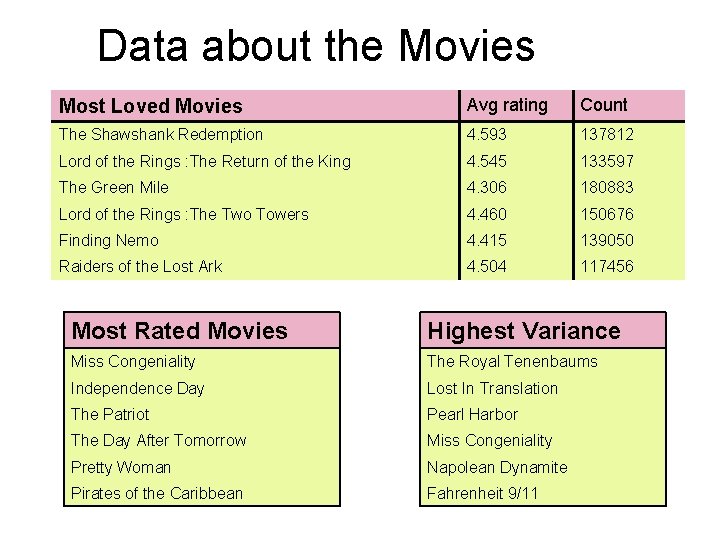
Data about the Movies Most Loved Movies Avg rating Count The Shawshank Redemption 4. 593 137812 Lord of the Rings : The Return of the King 4. 545 133597 The Green Mile 4. 306 180883 Lord of the Rings : The Two Towers 4. 460 150676 Finding Nemo 4. 415 139050 Raiders of the Lost Ark 4. 504 117456 Most Rated Movies Highest Variance Miss Congeniality The Royal Tenenbaums Independence Day Lost In Translation The Patriot Pearl Harbor The Day After Tomorrow Miss Congeniality Pretty Woman Napolean Dynamite Pirates of the Caribbean Fahrenheit 9/11

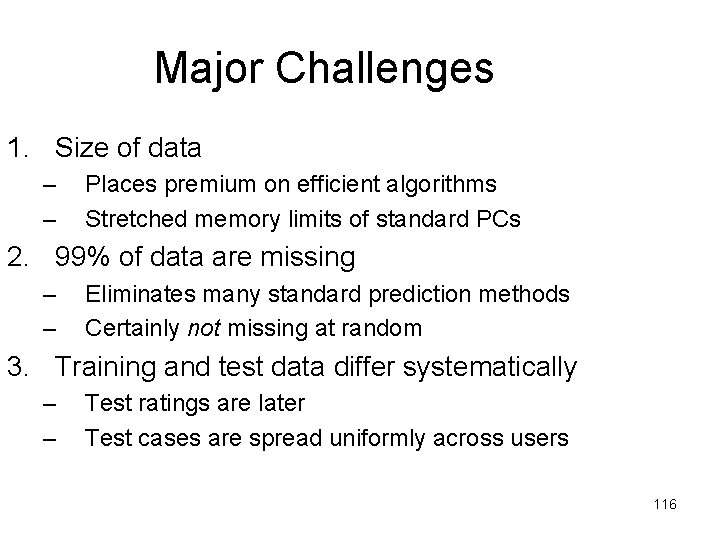
Major Challenges 1. Size of data – – Places premium on efficient algorithms Stretched memory limits of standard PCs 2. 99% of data are missing – – Eliminates many standard prediction methods Certainly not missing at random 3. Training and test data differ systematically – – Test ratings are later Test cases are spread uniformly across users 116

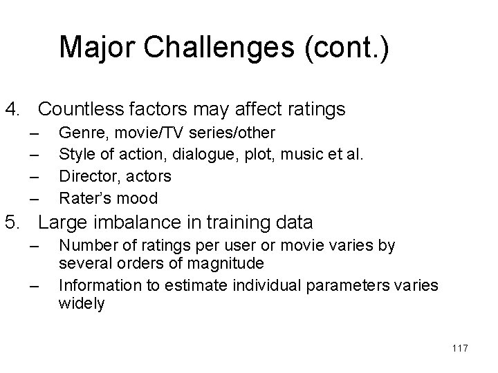
Major Challenges (cont. ) 4. Countless factors may affect ratings – – Genre, movie/TV series/other Style of action, dialogue, plot, music et al. Director, actors Rater’s mood 5. Large imbalance in training data – – Number of ratings per user or movie varies by several orders of magnitude Information to estimate individual parameters varies widely 117

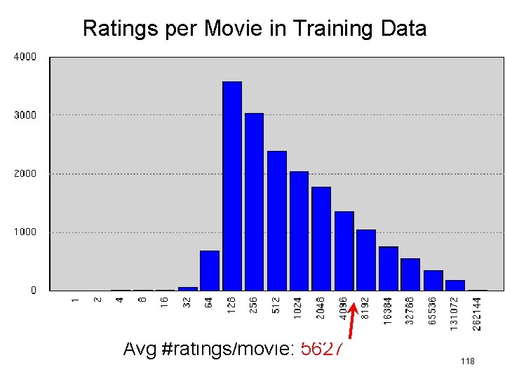
Ratings per Movie in Training Data Avg #ratings/movie: 5627 118

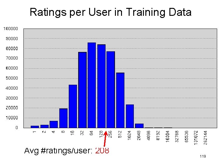
Ratings per User in Training Data Avg #ratings/user: 208 119

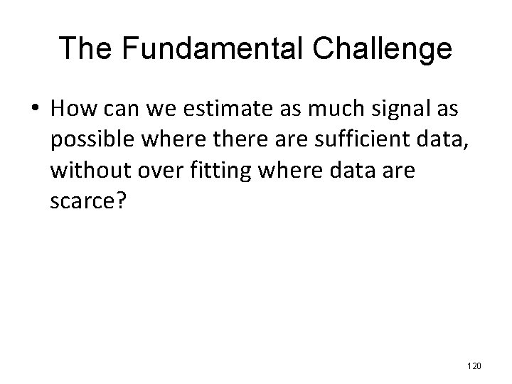
The Fundamental Challenge • How can we estimate as much signal as possible where there are sufficient data, without over fitting where data are scarce? 120

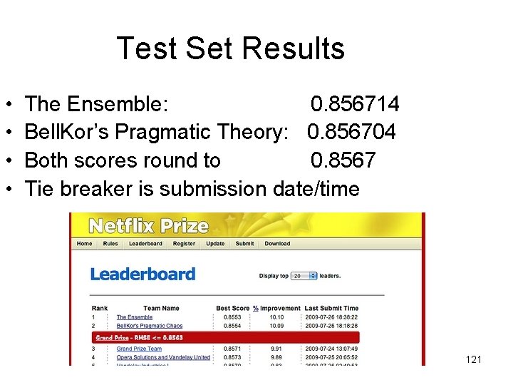
Test Set Results • • The Ensemble: 0. 856714 Bell. Kor’s Pragmatic Theory: 0. 856704 Both scores round to 0. 8567 Tie breaker is submission date/time 121

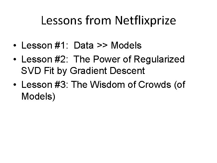
Lessons from Netflixprize • Lesson #1: Data >> Models • Lesson #2: The Power of Regularized SVD Fit by Gradient Descent • Lesson #3: The Wisdom of Crowds (of Models)

References • Koren, Yehuda. “Factorization meets the neighborhood: a multifaceted collaborative filtering model. ” In Proceeding of the 14 th ACM SIGKDD international conference on Knowledge discovery and data mining, 426– 434. ACM, 2008. http: //portal. acm. org/citation. cfm? id=1401890. 1401944 • Koren, Yehuda. “Collaborative filtering with temporal dynamics. ” Proceedings of the 15 th ACM SIGKDD international conference on Knowledge discovery and data mining - KDD ’ 09 (2009): 447. http: //portal. acm. org/citation. cfm? doid=1557019. 1557072. • Das, A. S. , M. Datar, A. Garg, and S. Rajaram. “Google news personalization: scalable online collaborative filtering. ” In Proceedings of the 16 th international conference on World Wide Web, 271– 280. ACM New York, NY, USA, 2007. http: //portal. acm. org/citation. cfm? id=1242610. • Linden, G. , B. Smith, and J. York. “Amazon. com recommendations: item-to-item collaborative filtering. ” IEEE Internet Computing 7, no. 1 (January 2003): 76 -80. http: //ieeexplore. ieee. org/lpdocs/epic 03/wrapper. htm? arnumber=1167344. • Davidson, James, Benjamin Liebald, and Taylor Van Vleet. “The You. Tube Video Recommendation System. ” Design (2010): 293 -296.