Line Fitting James Hayes Least squares line fitting

Line Fitting James Hayes

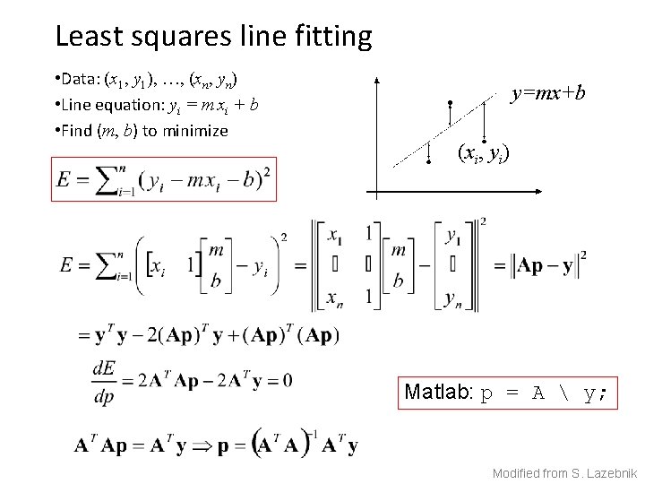
Least squares line fitting • Data: (x 1, y 1), …, (xn, yn) • Line equation: yi = m xi + b • Find (m, b) to minimize y=mx+b (xi, yi) Matlab: p = A y; Modified from S. Lazebnik

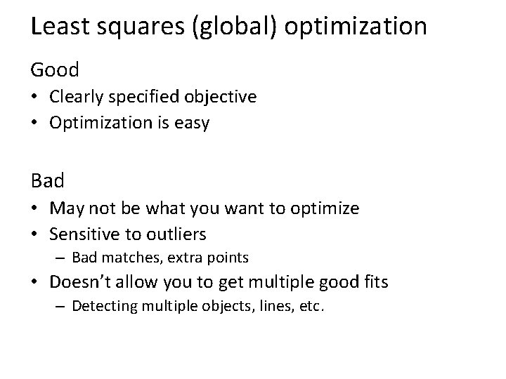
Least squares (global) optimization Good • Clearly specified objective • Optimization is easy Bad • May not be what you want to optimize • Sensitive to outliers – Bad matches, extra points • Doesn’t allow you to get multiple good fits – Detecting multiple objects, lines, etc.

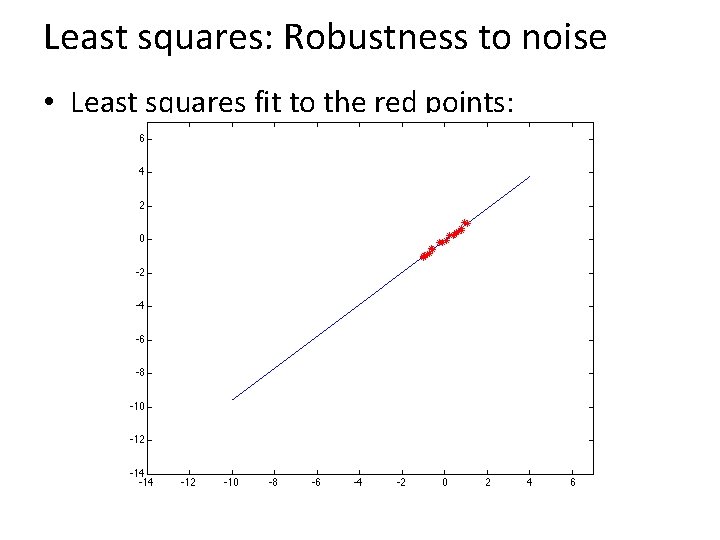
Least squares: Robustness to noise • Least squares fit to the red points:

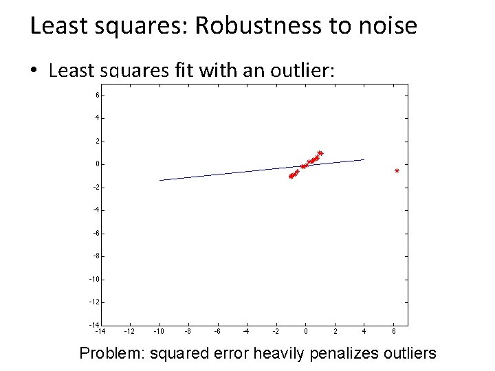
Least squares: Robustness to noise • Least squares fit with an outlier: Problem: squared error heavily penalizes outliers

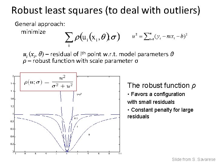
Robust least squares (to deal with outliers) General approach: minimize ui (xi, θ) – residual of ith point w. r. t. model parameters θ ρ – robust function with scale parameter σ The robust function ρ • Favors a configuration with small residuals • Constant penalty for large residuals Slide from S. Savarese

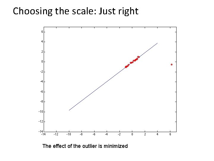
Choosing the scale: Just right The effect of the outlier is minimized

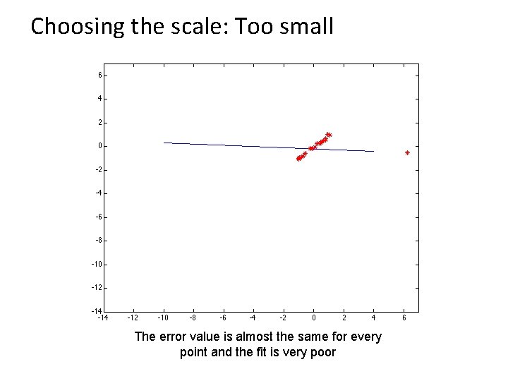
Choosing the scale: Too small The error value is almost the same for every point and the fit is very poor

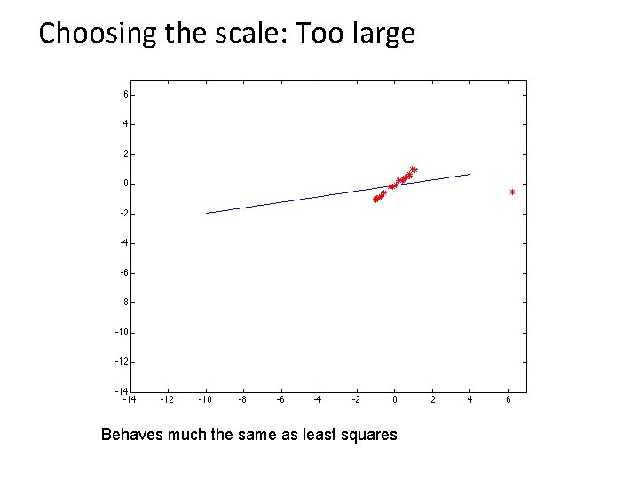
Choosing the scale: Too large Behaves much the same as least squares

Robust estimation: Details • Robust fitting is a nonlinear optimization problem that must be solved iteratively • Least squares solution can be used for initialization • Scale of robust function should be chosen adaptively based on median residual

Other ways to search for parameters (for when no closed form solution exists) • Line search 1. 2. • Grid search 1. 2. • For each parameter, step through values and choose value that gives best fit Repeat (1) until no parameter changes Propose several sets of parameters, evenly sampled in the joint set Choose best (or top few) and sample joint parameters around the current best; repeat Gradient descent 1. 2. Provide initial position (e. g. , random) Locally search for better parameters by following gradient

Hypothesize and test 1. Propose parameters – – – Try all possible Each point votes for all consistent parameters Repeatedly sample enough points to solve for parameters 2. Score the given parameters – Number of consistent points, possibly weighted by distance 3. Choose from among the set of parameters – Global or local maximum of scores 4. Possibly refine parameters using inliers

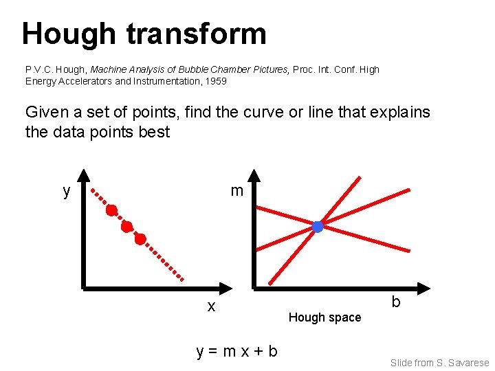
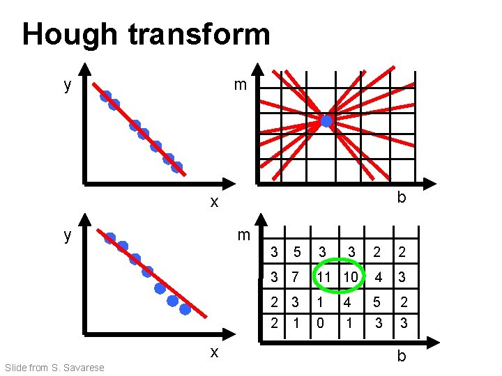
Hough Transform: Outline 1. Create a grid of parameter values 2. Each point votes for a set of parameters, incrementing those values in grid 3. Find maximum or local maxima in grid

Hough transform P. V. C. Hough, Machine Analysis of Bubble Chamber Pictures, Proc. Int. Conf. High Energy Accelerators and Instrumentation, 1959 Given a set of points, find the curve or line that explains the data points best y m x y=mx+b Hough space b Slide from S. Savarese

Hough transform y m b x y m 3 x Slide from S. Savarese 5 3 3 2 2 3 7 11 10 4 3 2 1 1 0 5 3 2 3 4 1 b

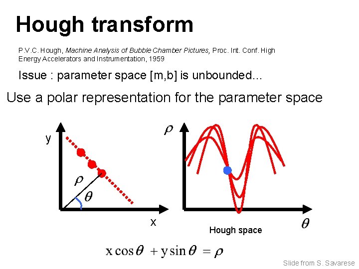
Hough transform P. V. C. Hough, Machine Analysis of Bubble Chamber Pictures, Proc. Int. Conf. High Energy Accelerators and Instrumentation, 1959 Issue : parameter space [m, b] is unbounded… Use a polar representation for the parameter space y x Hough space Slide from S. Savarese

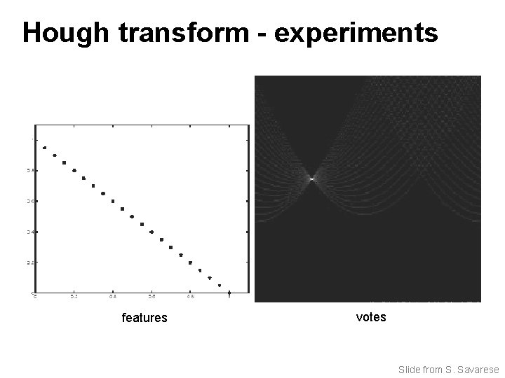
Hough transform - experiments features votes Slide from S. Savarese

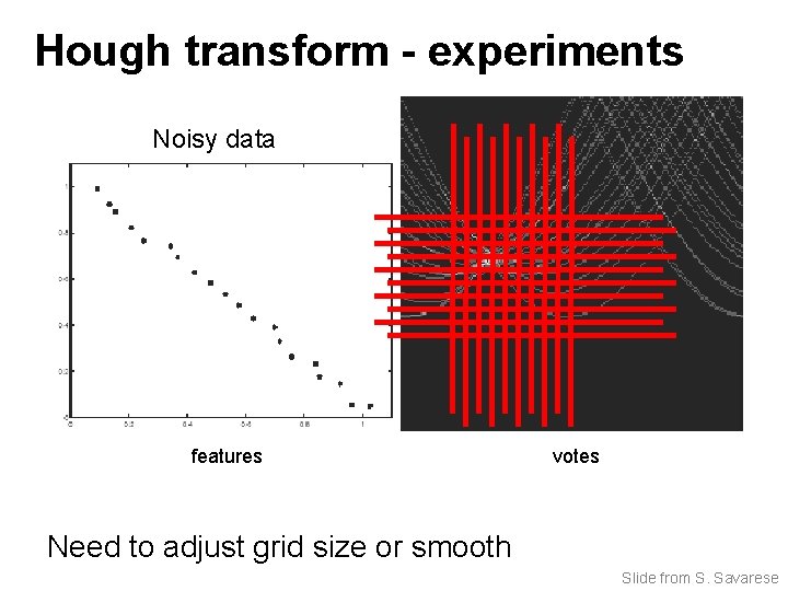
Hough transform - experiments Noisy data features votes Need to adjust grid size or smooth Slide from S. Savarese

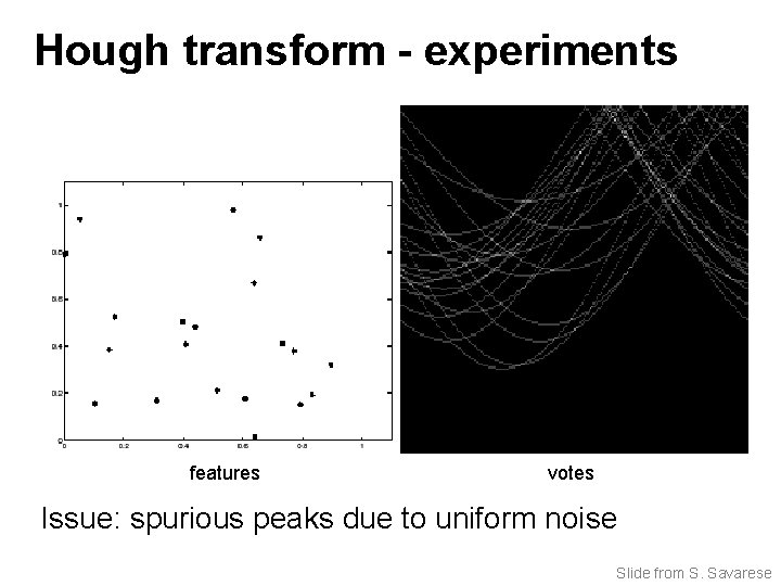
Hough transform - experiments features votes Issue: spurious peaks due to uniform noise Slide from S. Savarese

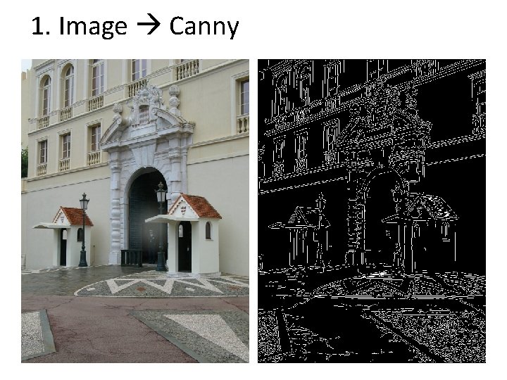
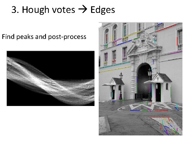
1. Image Canny

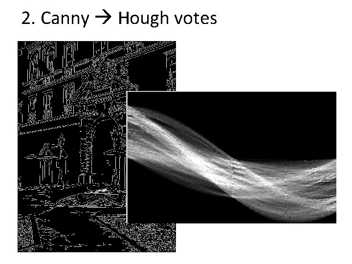
2. Canny Hough votes

3. Hough votes Edges Find peaks and post-process

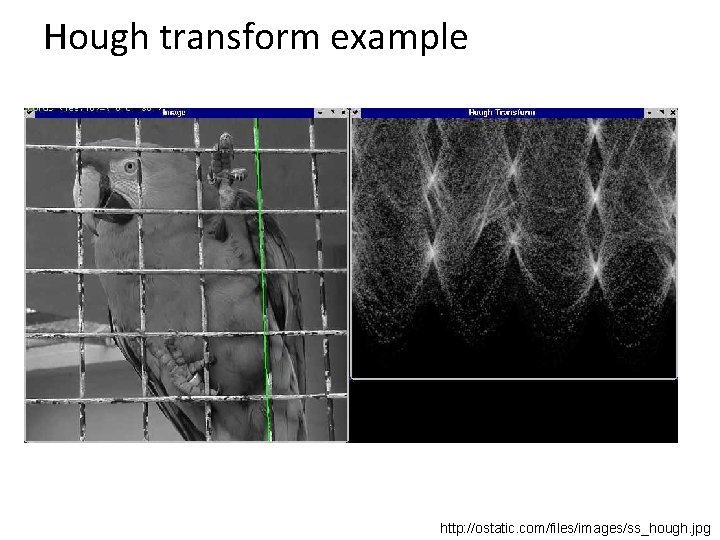
Hough transform example http: //ostatic. com/files/images/ss_hough. jpg

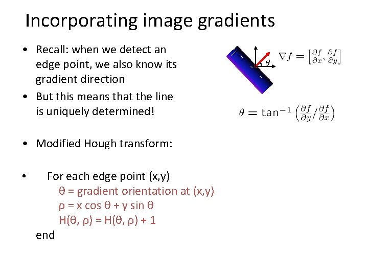
Incorporating image gradients • Recall: when we detect an edge point, we also know its gradient direction • But this means that the line is uniquely determined! • Modified Hough transform: • For each edge point (x, y) θ = gradient orientation at (x, y) ρ = x cos θ + y sin θ H(θ, ρ) = H(θ, ρ) + 1 end

Finding lines using Hough transform • Using m, b parameterization • Using r, theta parameterization – Using oriented gradients • Practical considerations – Bin size – Smoothing – Finding multiple lines – Finding line segments