Least Squares Fitting and Equation Solving with MPFIT

Least Squares Fitting and Equation Solving with MPFIT Craig Markwardt University of Maryland NASA’s Goddard Spaceflight Center http: //purl. com/net/mpfit 2009 -04 -15

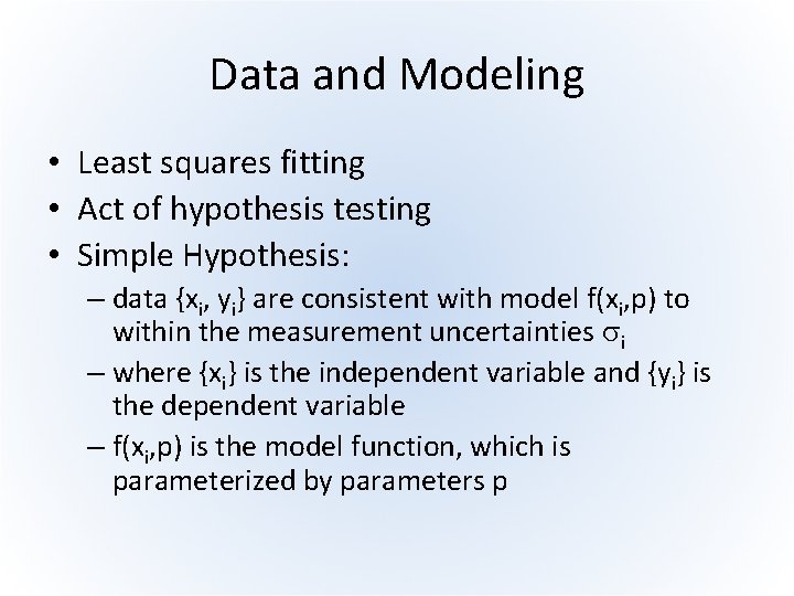
Data and Modeling • Least squares fitting • Act of hypothesis testing • Simple Hypothesis: – data {xi, yi} are consistent with model f(xi, p) to within the measurement uncertainties si – where {xi} is the independent variable and {yi} is the dependent variable – f(xi, p) is the model function, which is parameterized by parameters p

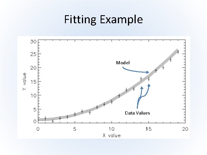
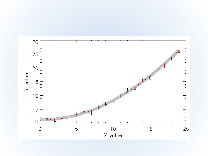
Fitting Example Model Data Values

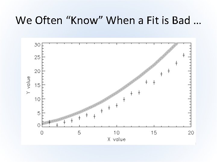
We Often “Know” When a Fit is Bad …

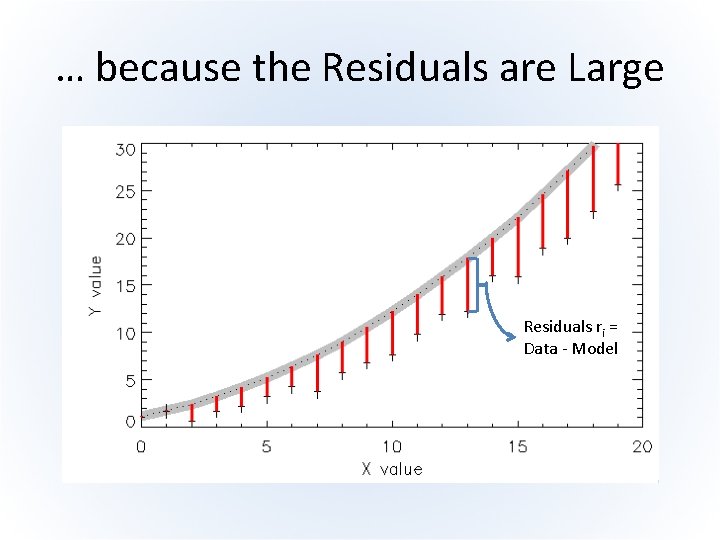
… because the Residuals are Large Residuals ri = Data - Model

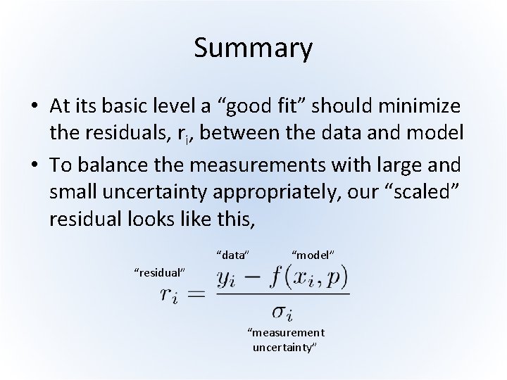
Summary • At its basic level a “good fit” should minimize the residuals, ri, between the data and model • To balance the measurements with large and small uncertainty appropriately, our “scaled” residual looks like this, “data” “model” “residual” “measurement uncertainty”

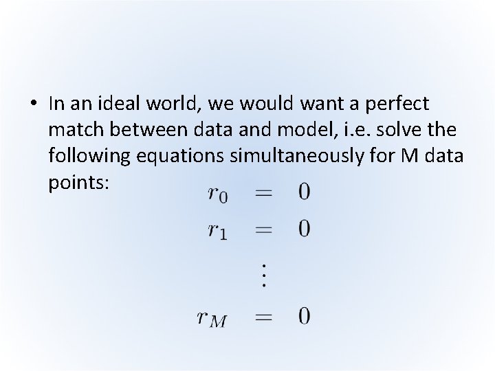
• In an ideal world, we would want a perfect match between data and model, i. e. solve the following equations simultaneously for M data points:

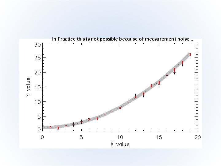
In Practice this is not possible because of measurement noise…

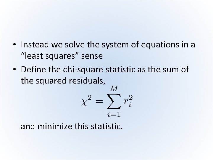
• Instead we solve the system of equations in a “least squares” sense • Define the chi-square statistic as the sum of the squared residuals, and minimize this statistic.

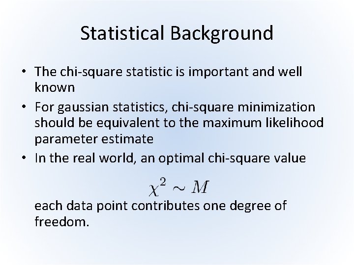
Statistical Background • The chi-square statistic is important and well known • For gaussian statistics, chi-square minimization should be equivalent to the maximum likelihood parameter estimate • In the real world, an optimal chi-square value each data point contributes one degree of freedom.

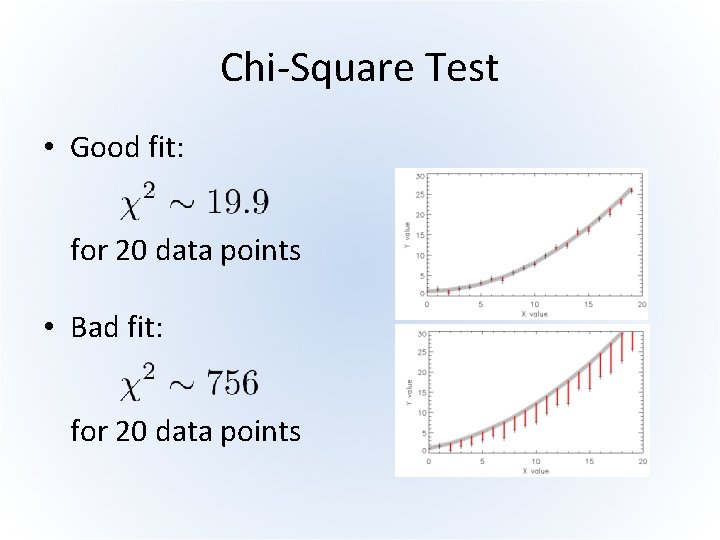
Chi-Square Test • Good fit: for 20 data points • Bad fit: for 20 data points

Existing Fitting Tools in IDL • General non-linear: – CURVEFIT – Bevington algorithm (vectorized) – LMFIT – Numerical recipes (not vectorized) • Specialized: – LINFIT – linear (y = ax + b) – POLY_FIT – polynomial – SVDFIT – linear combinations – GAUSSFIT – peak fitting

Introducing MPFIT • Powerful fitting engine based on MINPACK-1 (Moré and collaborators; http: //netlib. org/minpack/) • Robust factorization and stepping algorithms • Innovations: – Private data to user functions (FUNCTARGS) – Parameter upper and lower bounds (PARINFO) – User chooses who computes derivatives – Control over iteration, console output, stopping tolerances

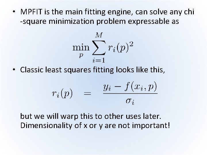
• MPFIT is the main fitting engine, can solve any chi -square minimization problem expressable as • Classic least squares fitting looks like this, but we will warp this to other uses later. Dimensionality of x or y are not important!

The MPFIT Family of Routines • Core fitting engine: MPFIT • 1 D Convenience routines: – MPFITFUN – MPFITEXPR – command line fitting – MPFITPEAK – peak fitting – MPCURVEFIT – drop-in replacement for CURVEFIT • 2 D Convenience routines: – MPFIT 2 DFUN – MPFIT 2 DPEAK – peak fitting

Simple Example: MPFITEXPR • Basic command line fitting, great for diagnosing data on the fly • You supply a model function expression – expr = 'P[0] + X*P[1] + X^2*P[2]’ • And then call MPFITEXPR “x” “y” “errors” “start values” – p = mpfitexpr(expr, xx, ys, ye, [1, 1, 1 d], …) • Demo (mpfit_expr. pro)

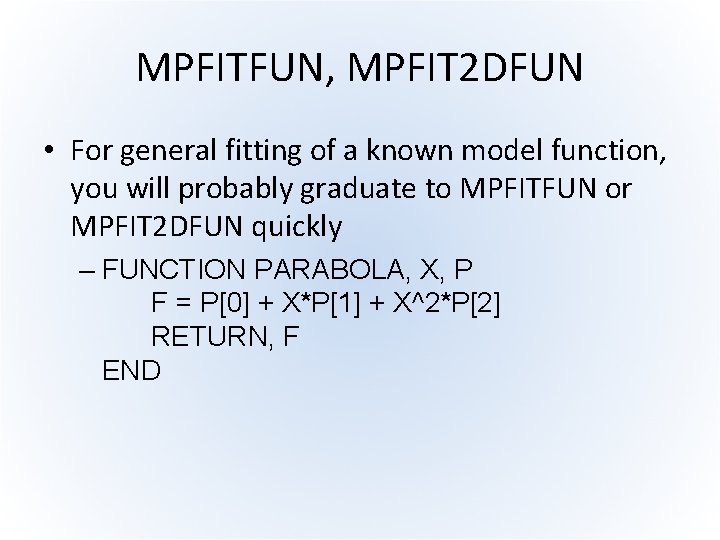
MPFITFUN, MPFIT 2 DFUN • For general fitting of a known model function, you will probably graduate to MPFITFUN or MPFIT 2 DFUN quickly – FUNCTION PARABOLA, X, P F = P[0] + X*P[1] + X^2*P[2] RETURN, F END

For More on the Basics • Setting parameter boundaries (PARINFO) • Passing private information (FUNCTARGS) • Retrieving best-fit model function and chisquare value (YFIT and BESTNORM) See my website

More Advanced Topics • Multi-dimensional data • Complicated constraints • Equation solving

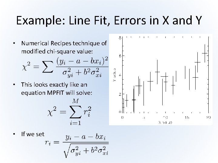
Example: Line Fit, Errors in X and Y • Numerical Recipes technique of modified chi-square value: • This looks exactly like an equation MPFIT will solve: • If we set

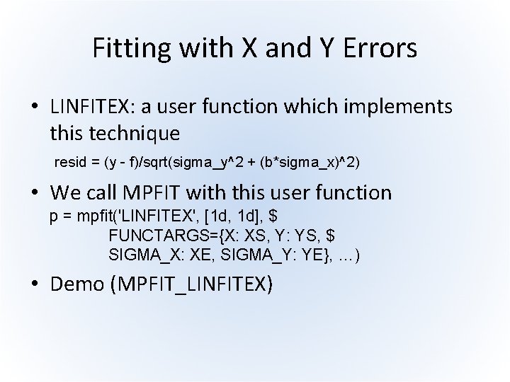
Fitting with X and Y Errors • LINFITEX: a user function which implements this technique resid = (y - f)/sqrt(sigma_y^2 + (b*sigma_x)^2) • We call MPFIT with this user function p = mpfit('LINFITEX', [1 d, 1 d], $ FUNCTARGS={X: XS, Y: YS, $ SIGMA_X: XE, SIGMA_Y: YE}, …) • Demo (MPFIT_LINFITEX)

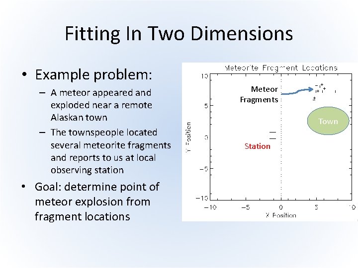
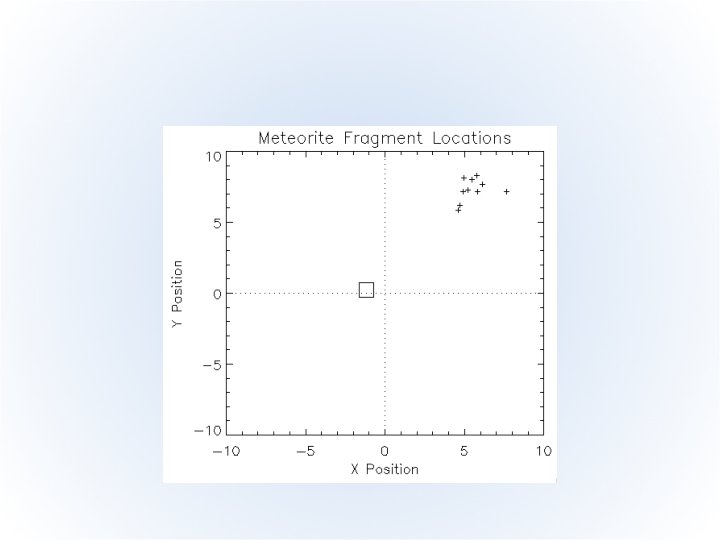
Fitting In Two Dimensions • Example problem: – A meteor appeared and exploded near a remote Alaskan town – The townspeople located several meteorite fragments and reports to us at local observing station • Goal: determine point of meteor explosion from fragment locations Meteor Fragments Town Station

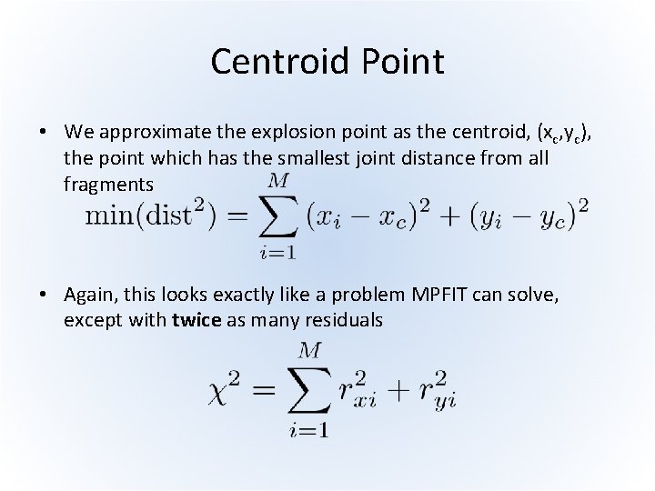
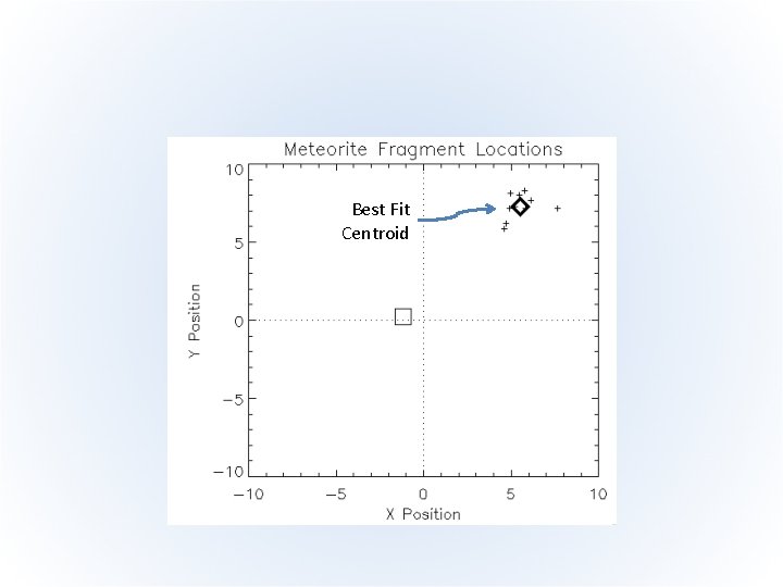
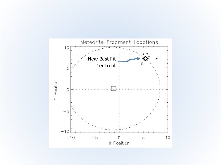
Centroid Point • We approximate the explosion point as the centroid, (xc, yc), the point which has the smallest joint distance from all fragments • Again, this looks exactly like a problem MPFIT can solve, except with twice as many residuals

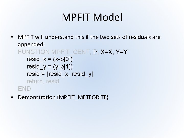
MPFIT Model • MPFIT will understand this if the two sets of residuals are appended: FUNCTION MPFIT_CENT, P, X=X, Y=Y resid_x = (x-p[0]) resid_y = (y-p[1]) resid = [resid_x, resid_y] return, resid END • Demonstration (MPFIT_METEORITE)

Best Fit Centroid

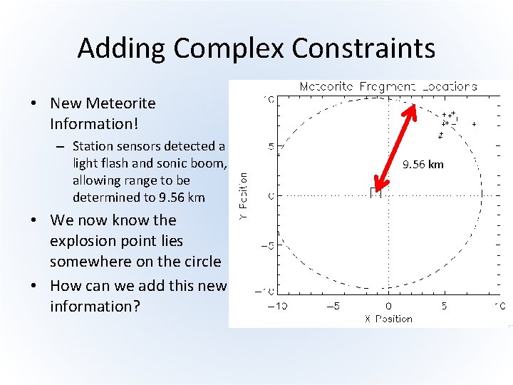
Adding Complex Constraints • New Meteorite Information! – Station sensors detected a light flash and sonic boom, allowing range to be determined to 9. 56 km • We now know the explosion point lies somewhere on the circle • How can we add this new information? 9. 56 km

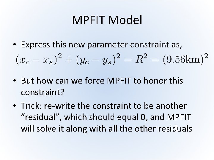
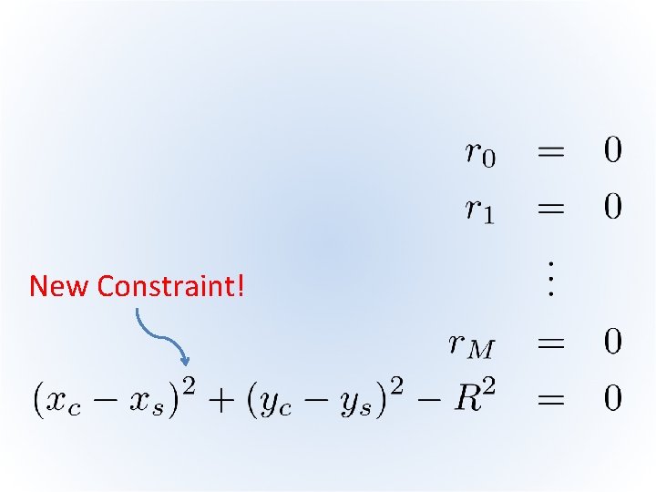
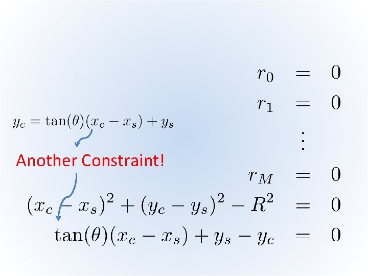
MPFIT Model • Express this new parameter constraint as, • But how can we force MPFIT to honor this constraint? • Trick: re-write the constraint to be another “residual”, which should equal 0, and MPFIT will solve it along with all the other residuals

New Constraint!

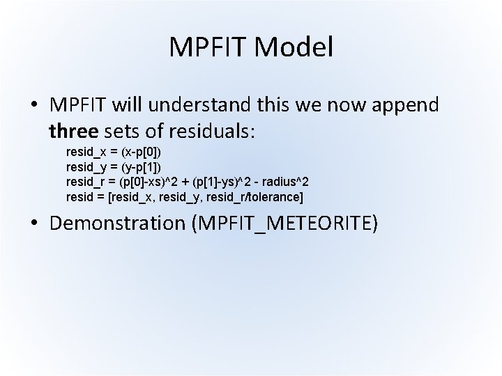
MPFIT Model • MPFIT will understand this we now append three sets of residuals: resid_x = (x-p[0]) resid_y = (y-p[1]) resid_r = (p[0]-xs)^2 + (p[1]-ys)^2 - radius^2 resid = [resid_x, resid_y, resid_r/tolerance] • Demonstration (MPFIT_METEORITE)

New Best Fit Centroid

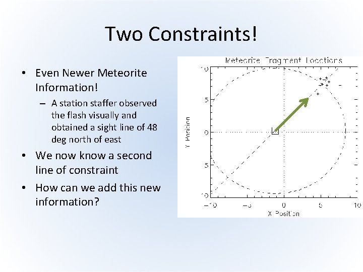
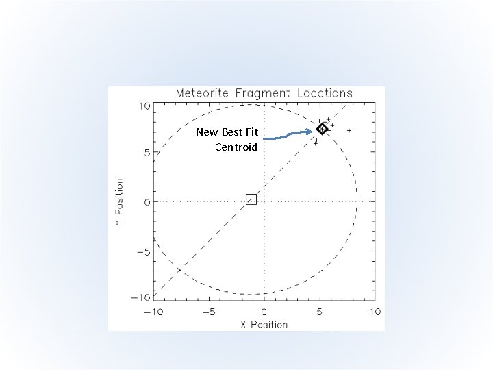
Two Constraints! • Even Newer Meteorite Information! – A station staffer observed the flash visually and obtained a sight line of 48 deg north of east • We now know a second line of constraint • How can we add this new information?

Another Constraint!

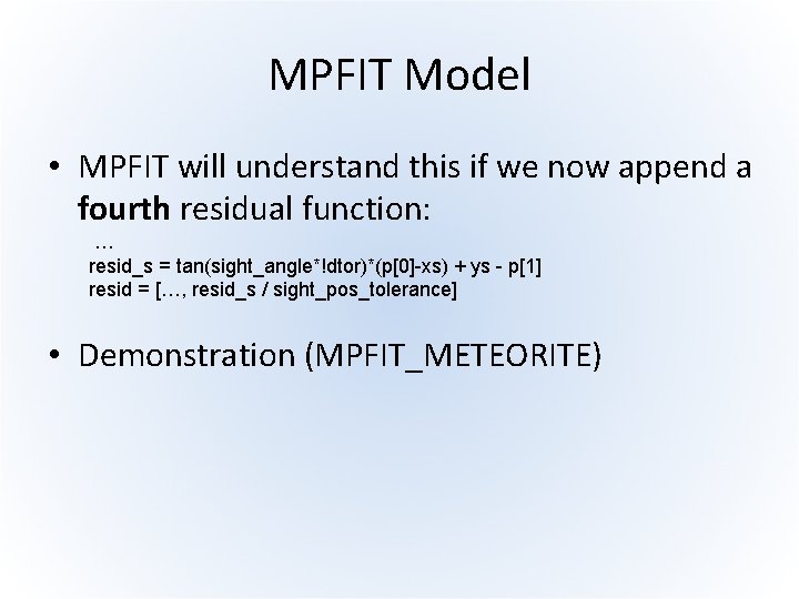
MPFIT Model • MPFIT will understand this if we now append a fourth residual function: … resid_s = tan(sight_angle*!dtor)*(p[0]-xs) + ys - p[1] resid = […, resid_s / sight_pos_tolerance] • Demonstration (MPFIT_METEORITE)

New Best Fit Centroid

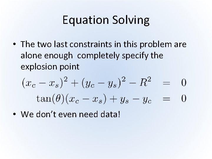
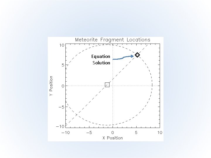
Equation Solving • The two last constraints in this problem are alone enough completely specify the explosion point • We don’t even need data!

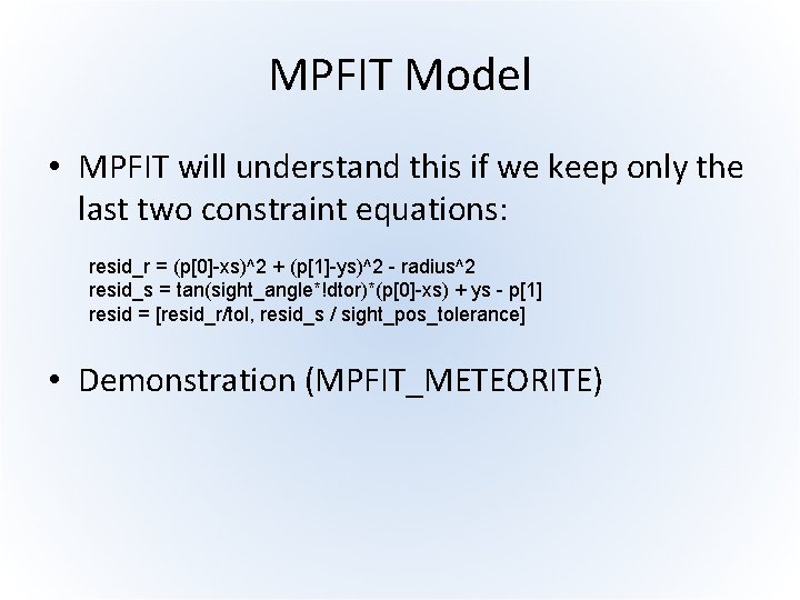
MPFIT Model • MPFIT will understand this if we keep only the last two constraint equations: resid_r = (p[0]-xs)^2 + (p[1]-ys)^2 - radius^2 resid_s = tan(sight_angle*!dtor)*(p[0]-xs) + ys - p[1] resid = [resid_r/tol, resid_s / sight_pos_tolerance] • Demonstration (MPFIT_METEORITE)

Equation Solution

Caveats • This technique depends on using MPFIT, not the other more “convenient” routines • If MPFIT finds a solution, that does not prove it is unique (could be multiple solutions!) – Depends on initial conditions • If equations are poorly behaved, MPFIT may get stuck – Need to adjust derivatives parameters via PARINFO

Take Away Messages • MPFIT is a power equation solver • Fitting M points is just solving M equations • Adding new constraints is straightforward, just add new “residual” equations – i. e. re-express constraint as (function) / (tolerance) = 0 • Other estimators like “least absolute deviation” (LAD) and Poisson likelihood can be solved by warping their equations to look like a sum of squared residuals

Getting MPFIT • IDL version: http: //purl. com/net/mpfit • C version at same site