9 Recursive Least Squares 1 Recursive identification Suppose

(9) Recursive Least Squares 1

Recursive identification • Suppose, at time instant n, we have a new output value y(n) and we want to calculate θˆ(n). • In off-line or batch identification, the whole data up to time n is used to compute θˆ(n) without exploiting the previous estimate θˆ(n-1). • In this case, the whole computations are repeated every time instant and the computational time and memory storage requirements increase with time as the data size getting larger. • We would like a way of efficiently recalculating the model each time we have new data. 2

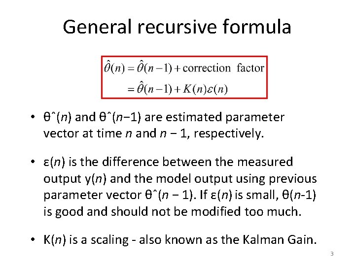
General recursive formula • θˆ(n) and θˆ(n− 1) are estimated parameter vector at time n and n − 1, respectively. • ε(n) is the difference between the measured output y(n) and the model output using previous parameter vector θˆ(n − 1). If ε(n) is small, θ(n-1) is good and should not be modified too much. • K(n) is a scaling - also known as the Kalman Gain. 3

Advantages of recursive estimation • Gives an estimate of the model from the first time step. • Computationally more efficient and less memory intensive, especially if we can avoid large matrix inverse calculations. • Ideal for real-time implementations. • Can adapt to changing systems → forms the core of adaptive control and signal processing. 4

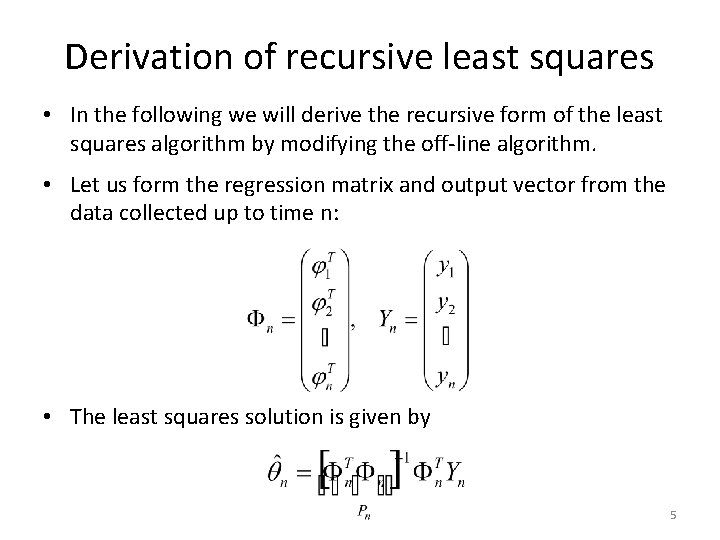
Derivation of recursive least squares • In the following we will derive the recursive form of the least squares algorithm by modifying the off-line algorithm. • Let us form the regression matrix and output vector from the data collected up to time n: • The least squares solution is given by 5

Derivation of recursive least squares • Let’s look at the expression for 6

7

Yet we still need a matrix inverse in (6) which is computationally expensive. This can be avoided using the matrix inversion lemma 8

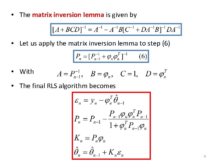
• The matrix inversion lemma is given by • Let us apply the matrix inversion lemma to step (6) • With • The final RLS algorithm becomes 9

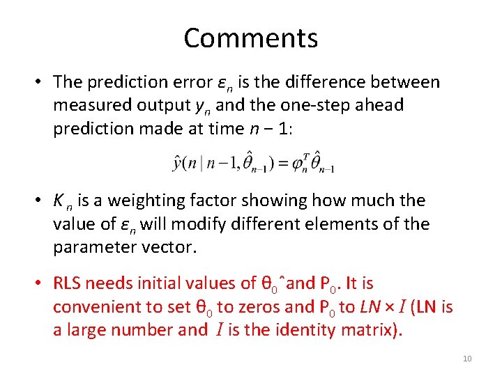
Comments • The prediction error εn is the difference between measured output yn and the one-step ahead prediction made at time n − 1: • K n is a weighting factor showing how much the value of εn will modify different elements of the parameter vector. • RLS needs initial values of θ 0ˆand P 0. It is convenient to set θ 0 to zeros and P 0 to LN × I (LN is a large number and I is the identity matrix). 10

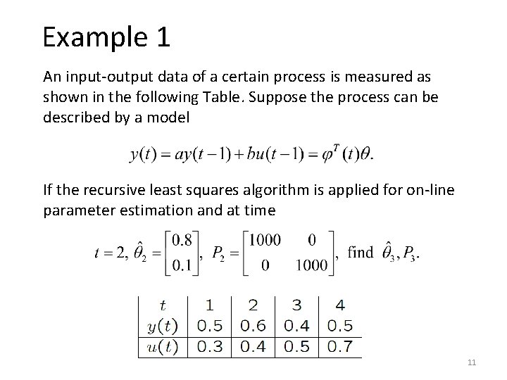
Example 1 An input-output data of a certain process is measured as shown in the following Table. Suppose the process can be described by a model If the recursive least squares algorithm is applied for on-line parameter estimation and at time 11

12

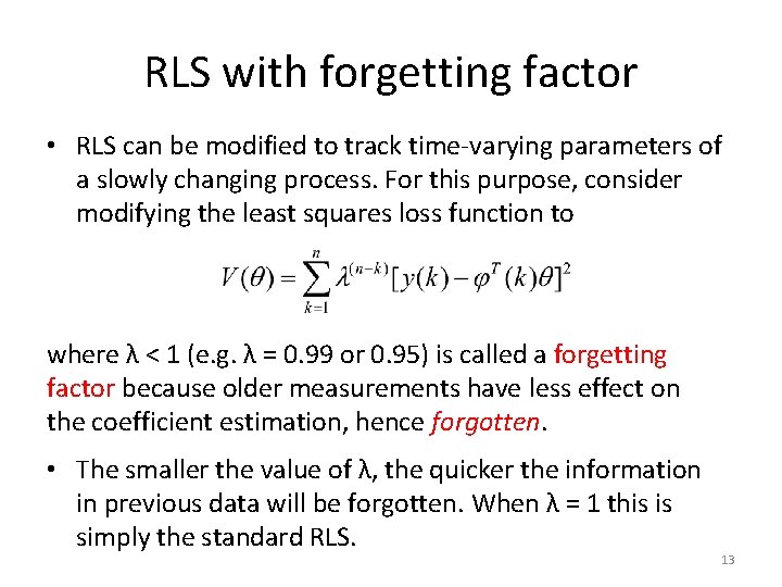
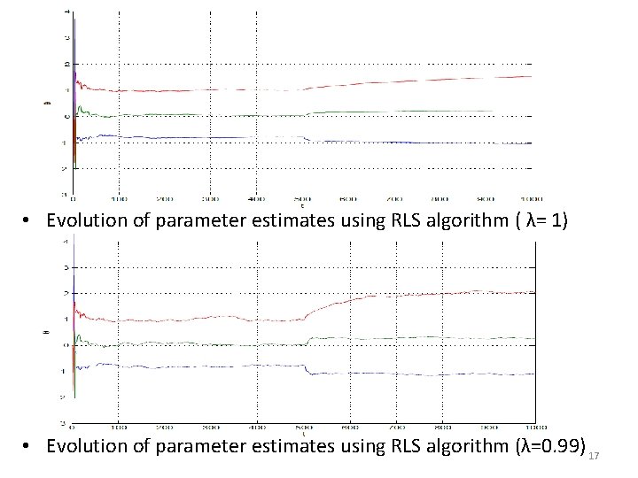
RLS with forgetting factor • RLS can be modified to track time-varying parameters of a slowly changing process. For this purpose, consider modifying the least squares loss function to where λ < 1 (e. g. λ = 0. 99 or 0. 95) is called a forgetting factor because older measurements have less effect on the coefficient estimation, hence forgotten. • The smaller the value of λ, the quicker the information in previous data will be forgotten. When λ = 1 this is simply the standard RLS. 13

RLS with forgetting factor 14

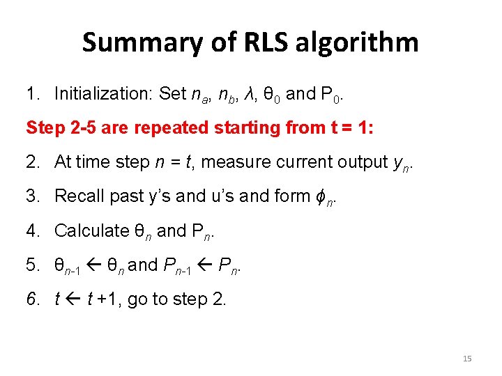
Summary of RLS algorithm 1. Initialization: Set na, nb, λ, θ 0 and P 0. Step 2 -5 are repeated starting from t = 1: 2. At time step n = t, measure current output yn. 3. Recall past y’s and u’s and form ϕn. 4. Calculate θn and Pn. 5. θn-1 θn and Pn-1 Pn. 6. t t +1, go to step 2. 15

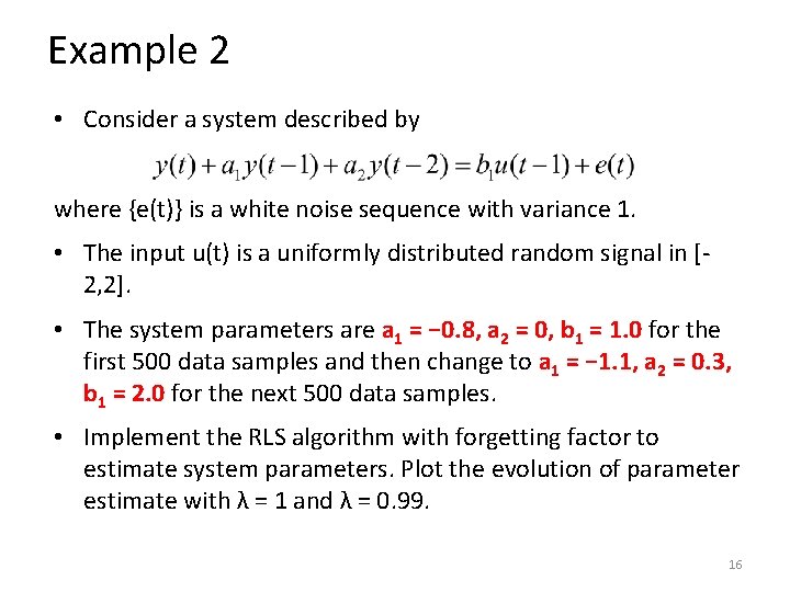
Example 2 • Consider a system described by where {e(t)} is a white noise sequence with variance 1. • The input u(t) is a uniformly distributed random signal in [2, 2]. • The system parameters are a 1 = − 0. 8, a 2 = 0, b 1 = 1. 0 for the first 500 data samples and then change to a 1 = − 1. 1, a 2 = 0. 3, b 1 = 2. 0 for the next 500 data samples. • Implement the RLS algorithm with forgetting factor to estimate system parameters. Plot the evolution of parameter estimate with λ = 1 and λ = 0. 99. 16

• Evolution of parameter estimates using RLS algorithm ( λ= 1) • Evolution of parameter estimates using RLS algorithm (λ=0. 99) 17

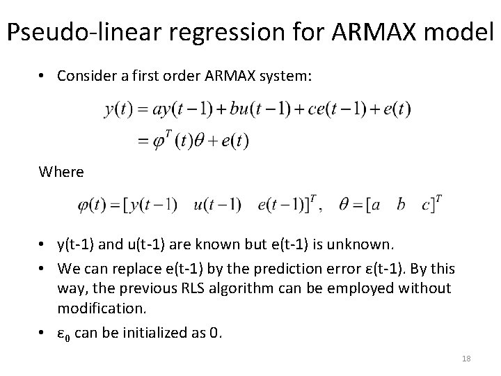
Pseudo-linear regression for ARMAX model • Consider a first order ARMAX system: Where • y(t-1) and u(t-1) are known but e(t-1) is unknown. • We can replace e(t-1) by the prediction error ε(t-1). By this way, the previous RLS algorithm can be employed without modification. • ε 0 can be initialized as 0. 18