3 2 Least Squares Regression Line Regression Line

3. 2 Least Squares Regression Line

Regression Line • Describes how a response variable changes as an explanatory variable changes • Formula sheet: • Calculator version:

Slope • Formula Sheet • Interpretation: how will the predicted response variable change for one increase in the explanatory variable?

Y-Intercept • Formula Sheet • Interpretation: what is the predicted response variable if there is no explanatory variable? • Mathematically - needed! • Realistically - might not make sense! • Sometimes the explanatory variable might not make sense being zero

context of the problem. Determine if the yintercept is realistic for this problem, explain. (I will write the equation on the board)

Extrapolation • When using a regression line to predict a variable outside the range of the data gathered • Unreliable predictions!

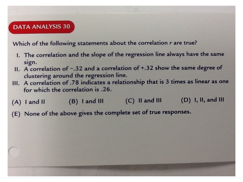
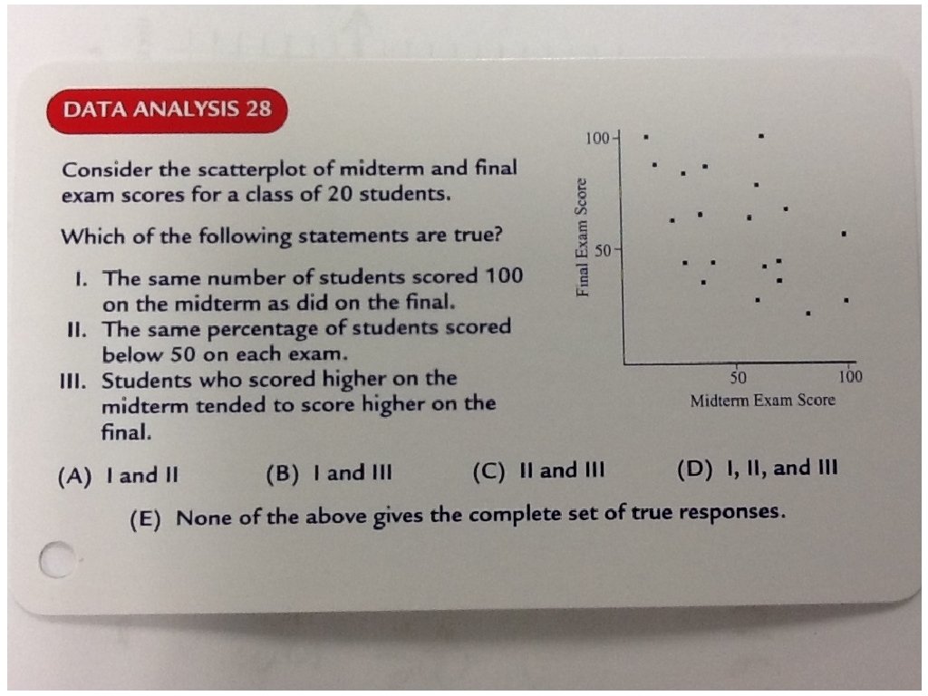
Multiple Choice Problems

Let's do p. 160!

3. 2 - Least. Squares Regression (Residuals)

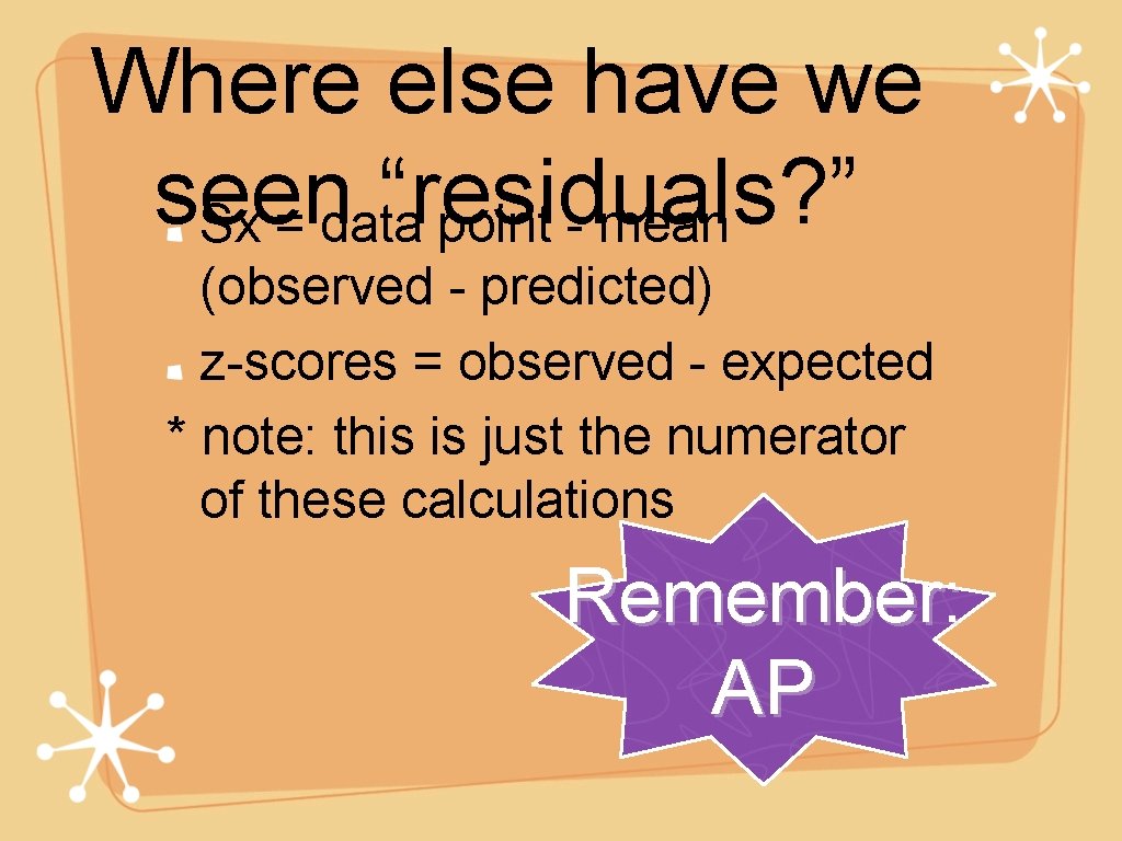
Where else have we seen “residuals? ” Sx = data point - mean (observed - predicted) z-scores = observed - expected * note: this is just the numerator of these calculations Remember: AP

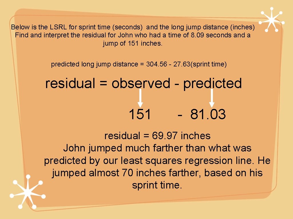
Below is the LSRL for sprint time (seconds) and the long jump distance (inches) Find and interpret the residual for John who had a time of 8. 09 seconds and a jump of 151 inches. predicted long jump distance = 304. 56 - 27. 63(sprint time) residual = observed - predicted 151 - 81. 03 residual = 69. 97 inches John jumped much farther than what was predicted by our least squares regression line. He jumped almost 70 inches farther, based on his sprint time.

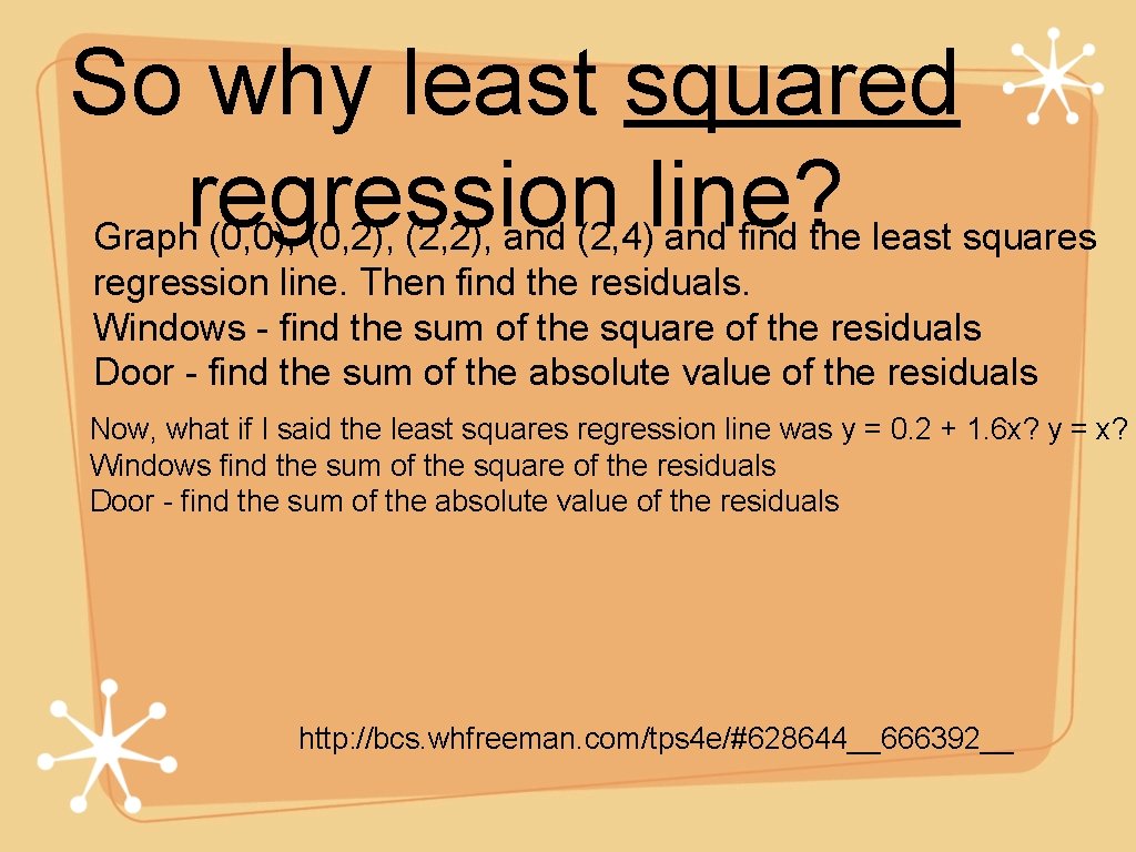
So why least squared regression line? Graph (0, 0), (0, 2), (2, 2), and (2, 4) and find the least squares regression line. Then find the residuals. Windows - find the sum of the square of the residuals Door - find the sum of the absolute value of the residuals Now, what if I said the least squares regression line was y = 0. 2 + 1. 6 x? y = x? Windows find the sum of the square of the residuals Door - find the sum of the absolute value of the residuals http: //bcs. whfreeman. com/tps 4 e/#628644__666392__

Stop notes for today Homework is p 193 #43, 45, 47, 53 Activity - "Matching Descriptions to Scatterplots" Homework hint: you will need to be familiar with the formulas on your sheet to write the LSRL

Residual Plots a scatterplot of the residuals against the explanatory variable. used to help assess the strength of your regression line

Residual Plots with Normal Probability Plots we want the graphs to be linear to support the Normality of our data. with Residual Plots we want the residuals to be very scattered so our data is can be model with a linear regression. Remember: Correlation does NOT assess linearity, just strength and direction!

What’s a Good Residual Plot? No obvious pattern - the LSRL would be in the middle of the data, some data above and some below Relatively small residuals - the data points are close to the LSRL

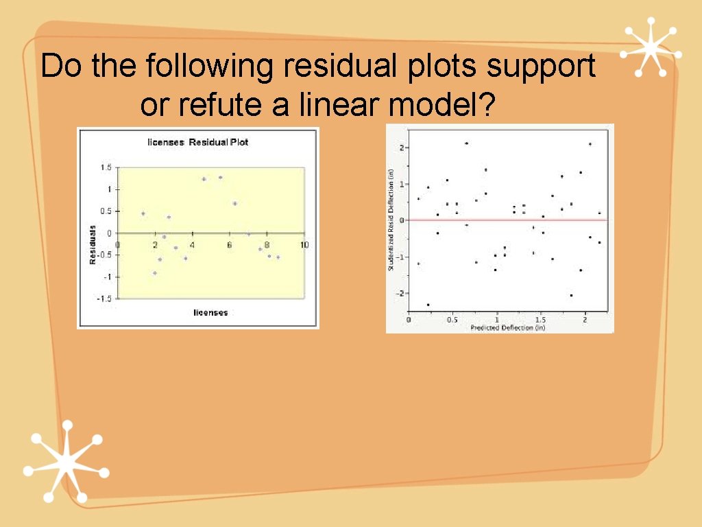
Do the following residual plots support or refute a linear model?

http: //content. ebscohost. com/pdf 23_24/pdf/2009/D 8 Y/01 Sep 09/43669525. pdf? T=P&P=AN&K=43669525&S=R&D=aph&Ebsco. Content=d. GJy. MNHX 8 k. Seq. K 84 y. Ovq. OLCmr 0 qep 7 RSs 6%2 B 4 S 7 a. Wx. WXS&Content. Custome ssk 2 xq. LJNue. Pfgeyx 44 Hy

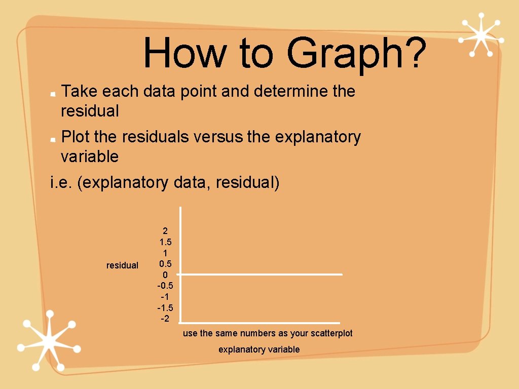
How to Graph? Take each data point and determine the residual Plot the residuals versus the explanatory variable i. e. (explanatory data, residual) residual 2 1. 5 1 0. 5 0 -0. 5 -1 -1. 5 -2 use the same numbers as your scatterplot explanatory variable

Calculator Construction If you have a lot of data, follow the instructions on page 178 to construct your residual plot (you will also have to have done the technology corner on p. 170)

What is Standard Deviation? the average squared distance a data point is from the mean Is there a sx? Is there a sy? So why not s? (standard deviation of residuals)

Standard Deviation of Residuals gives the approximate size of an “average” or “typical” prediction error from our LSRL formula on page 177 Why divide by n-2?