GPS time series construction Least Squares fitting Helmert

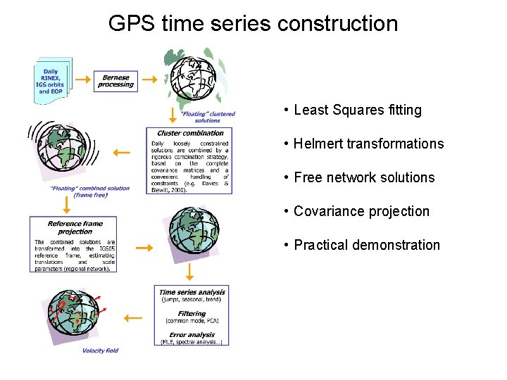
GPS time series construction • Least Squares fitting • Helmert transformations • Free network solutions • Covariance projection • Practical demonstration

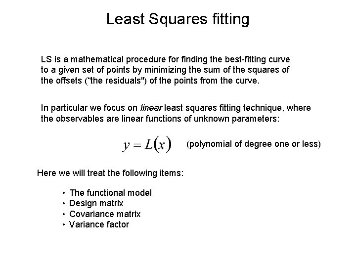
Least Squares fitting LS is a mathematical procedure for finding the best-fitting curve to a given set of points by minimizing the sum of the squares of the offsets (“the residuals") of the points from the curve. In particular we focus on linear least squares fitting technique, where the observables are linear functions of unknown parameters: (polynomial of degree one or less) Here we will treat the following items: • • The functional model Design matrix Covariance matrix Variance factor

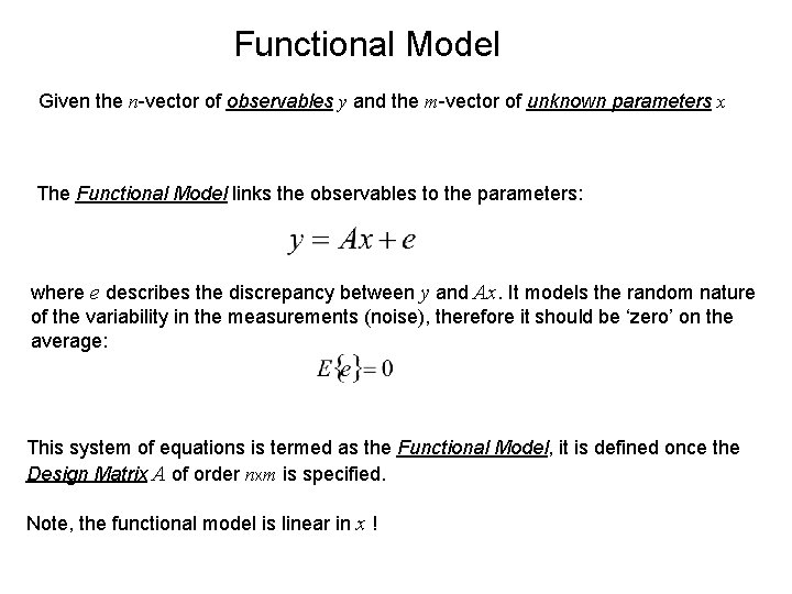
Functional Model Given the n-vector of observables y and the m-vector of unknown parameters x The Functional Model links the observables to the parameters: where e describes the discrepancy between y and Ax. It models the random nature of the variability in the measurements (noise), therefore it should be ‘zero’ on the average: This system of equations is termed as the Functional Model, it is defined once the Design Matrix A of order nxm is specified. Note, the functional model is linear in x !

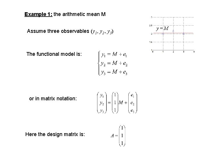
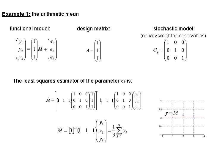
Example 1: the arithmetic mean M Assume three observables (y 1, y 2, y 3) The functional model is: or in matrix notation: Here the design matrix is: y=M

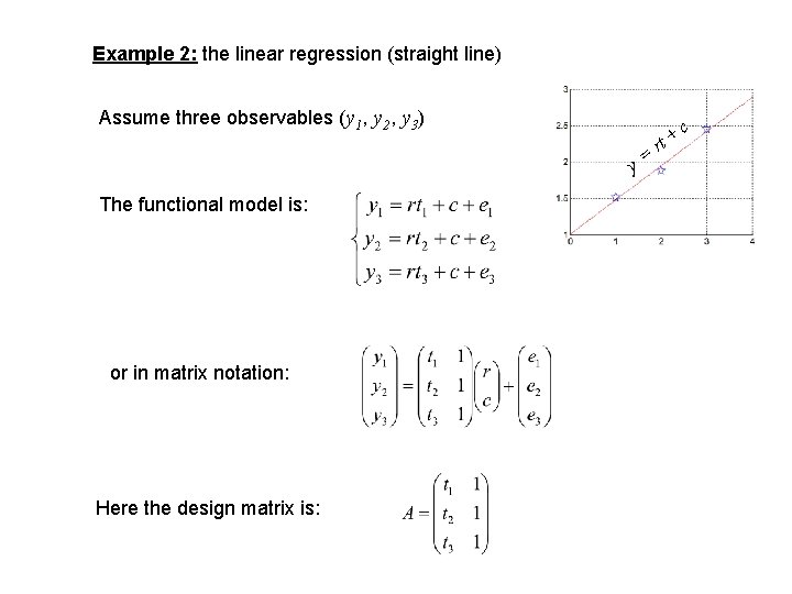
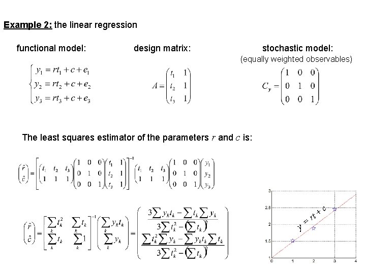
Example 2: the linear regression (straight line) Assume three observables (y 1, y 2, y 3) y= The functional model is: or in matrix notation: Here the design matrix is: rt + c

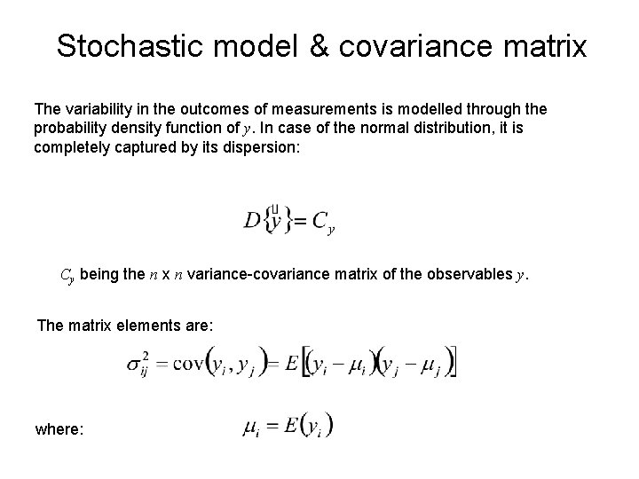
Stochastic model & covariance matrix The variability in the outcomes of measurements is modelled through the probability density function of y. In case of the normal distribution, it is completely captured by its dispersion: Cy being the n x n variance-covariance matrix of the observables y. The matrix elements are: where:

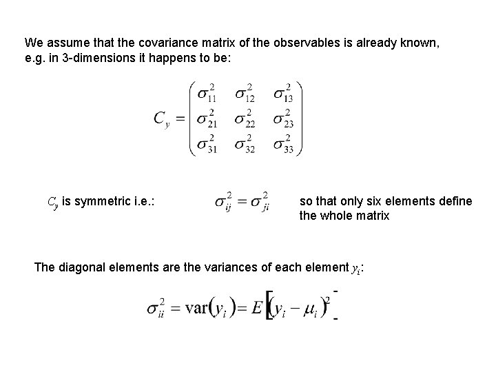
We assume that the covariance matrix of the observables is already known, e. g. in 3 -dimensions it happens to be: Cy is symmetric i. e. : so that only six elements define the whole matrix The diagonal elements are the variances of each element yi:

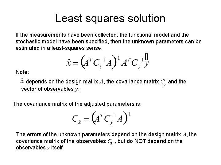
Least squares solution If the measurements have been collected, the functional model and the stochastic model have been specified, then the unknown parameters can be estimated in a least-squares sense: Note: depends on the design matrix A, the covariance matrix Cy and the vector of observables y. The covariance matrix of the adjusted parameters is: The errors of the unknown parameters depend on the design matrix A, the covariance matrix of the observables Cy , but do NOT depend on the observables y itself

Example 1: the arithmetic mean functional model: design matrix: stochastic model: (equally weighted observables) The least squares estimator of the parameter m is: y=M

Example 2: the linear regression functional model: design matrix: stochastic model: (equally weighted observables) The least squares estimator of the parameters r and c is: y= rt + c

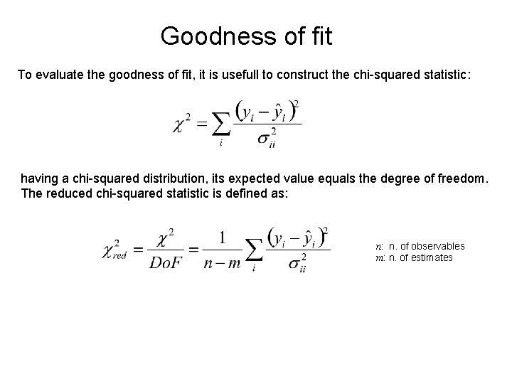
Goodness of fit To evaluate the goodness of fit, it is usefull to construct the chi-squared statistic: having a chi-squared distribution, its expected value equals the degree of freedom. The reduced chi-squared statistic is defined as: n: n. of observables m: n. of estimates

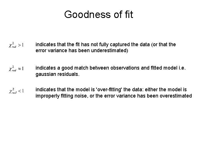
Goodness of fit indicates that the fit has not fully captured the data (or that the error variance has been underestimated) indicates a good match between observations and fitted model i. e. gaussian residuals. indicates that the model is 'over-fitting' the data: either the model is improperly fitting noise, or the error variance has been overestimated

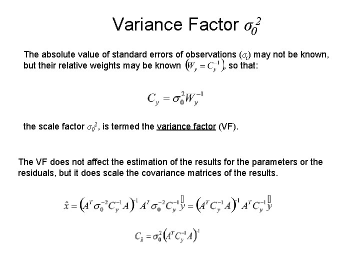
Variance Factor σ02 The absolute value of standard errors of observations (σi) may not be known, but their relative weights may be known , so that: the scale factor σ02, is termed the variance factor (VF). The VF does not affect the estimation of the results for the parameters or the residuals, but it does scale the covariance matrices of the results.

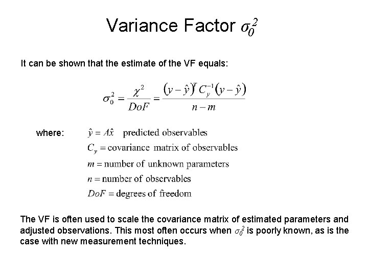
Variance Factor σ02 It can be shown that the estimate of the VF equals: where: The VF is often used to scale the covariance matrix of estimated parameters and adjusted observations. This most often occurs when σ02 is poorly known, as is the case with new measurement techniques.

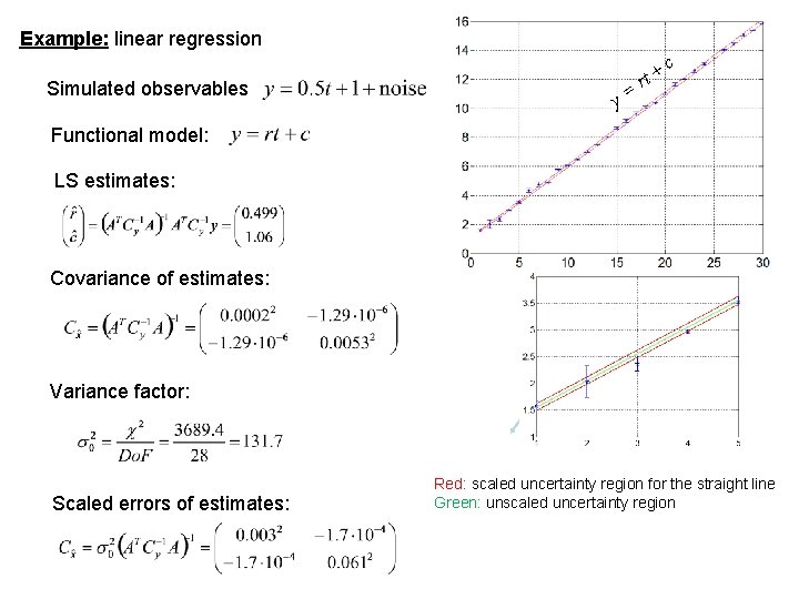
Example: linear regression Simulated observables y= rt + c Functional model: LS estimates: Covariance of estimates: Variance factor: Scaled errors of estimates: Red: scaled uncertainty region for the straight line Green: unscaled uncertainty region

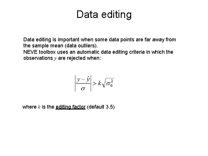
Data editing is important when some data points are far away from the sample mean (data outliers). NEVE toolbox uses an automatic data editing criteria in which the observations y are rejected when: where k is the editing factor (default 3. 5)

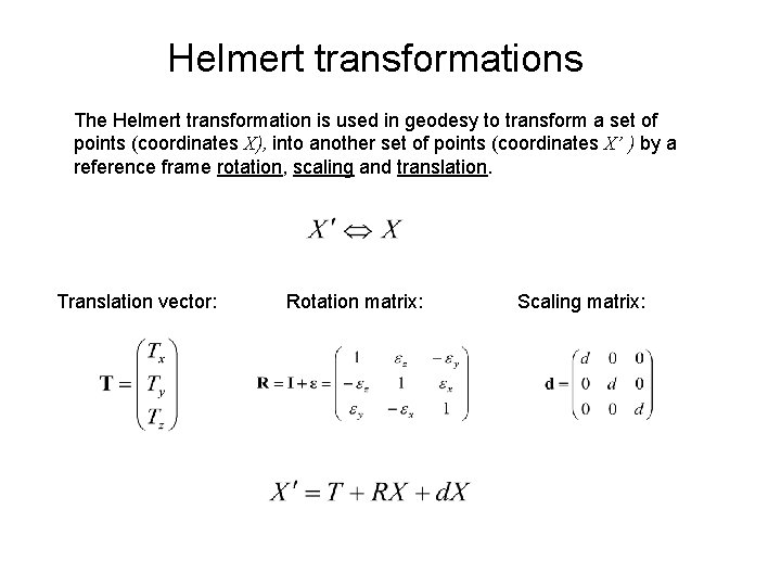
Helmert transformations The Helmert transformation is used in geodesy to transform a set of points (coordinates X), into another set of points (coordinates X’ ) by a reference frame rotation, scaling and translation. Translation vector: Rotation matrix: Scaling matrix:

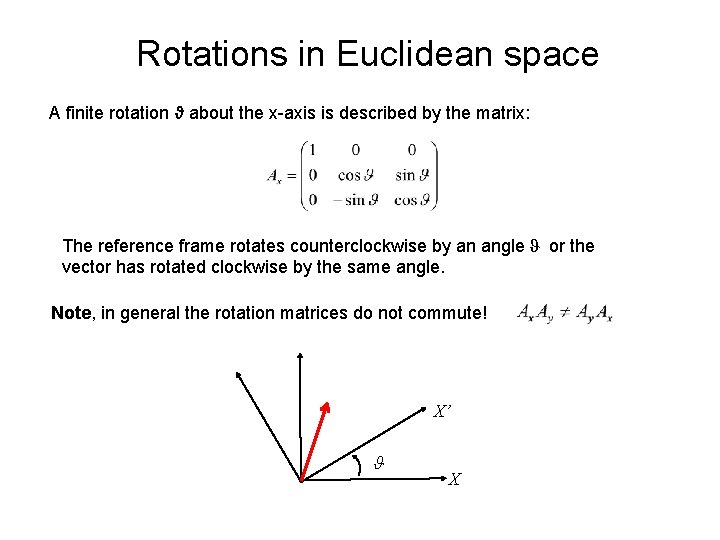
Rotations in Euclidean space A finite rotation ϑ about the x-axis is described by the matrix: The reference frame rotates counterclockwise by an angle ϑ or the vector has rotated clockwise by the same angle. Note, in general the rotation matrices do not commute! X’ ϑ X

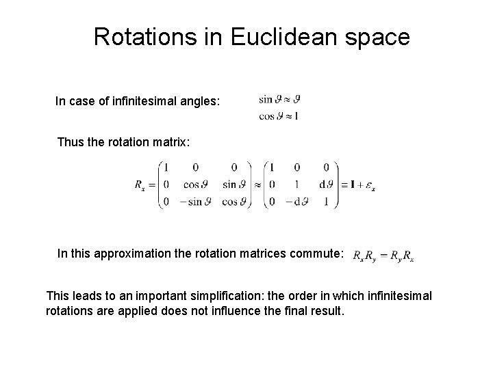
Rotations in Euclidean space In case of infinitesimal angles: Thus the rotation matrix: In this approximation the rotation matrices commute: This leads to an important simplification: the order in which infinitesimal rotations are applied does not influence the final result.

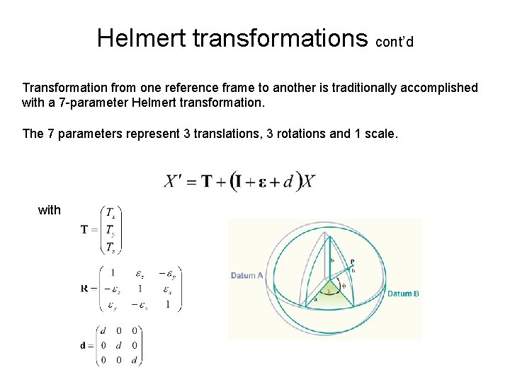
Helmert transformations cont’d Transformation from one reference frame to another is traditionally accomplished with a 7 -parameter Helmert transformation. The 7 parameters represent 3 translations, 3 rotations and 1 scale. with

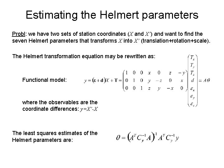
Estimating the Helmert parameters Probl: we have two sets of station coordinates (X and X’) and want to find the seven Helmert parameters that transforms X into X’ (translation+rotation+scale). The Helmert transformation equation may be rewritten as: Functional model: where the observables are the coordinate differences: y=X’-X The least squares estimates of the Helmert parameters are:

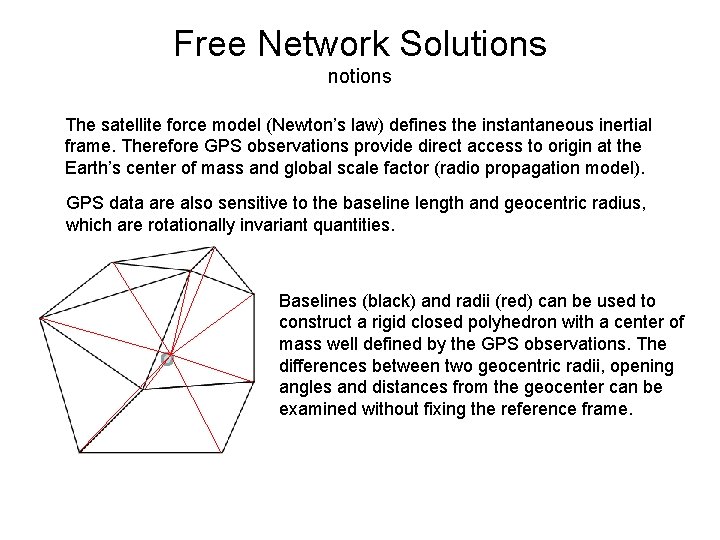
Free Network Solutions notions The satellite force model (Newton’s law) defines the instantaneous inertial frame. Therefore GPS observations provide direct access to origin at the Earth’s center of mass and global scale factor (radio propagation model). GPS data are also sensitive to the baseline length and geocentric radius, which are rotationally invariant quantities. Baselines (black) and radii (red) can be used to construct a rigid closed polyhedron with a center of mass well defined by the GPS observations. The differences between two geocentric radii, opening angles and distances from the geocenter can be examined without fixing the reference frame.

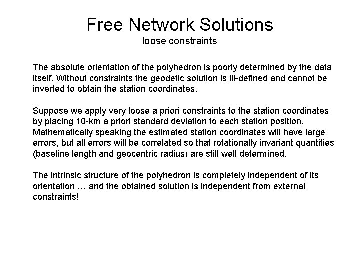
Free Network Solutions loose constraints The absolute orientation of the polyhedron is poorly determined by the data itself. Without constraints the geodetic solution is ill-defined and cannot be inverted to obtain the station coordinates. Suppose we apply very loose a priori constraints to the station coordinates by placing 10 -km a priori standard deviation to each station position. Mathematically speaking the estimated station coordinates will have large errors, but all errors will be correlated so that rotationally invariant quantities (baseline length and geocentric radius) are still well determined. The intrinsic structure of the polyhedron is completely independent of its orientation … and the obtained solution is independent from external constraints!

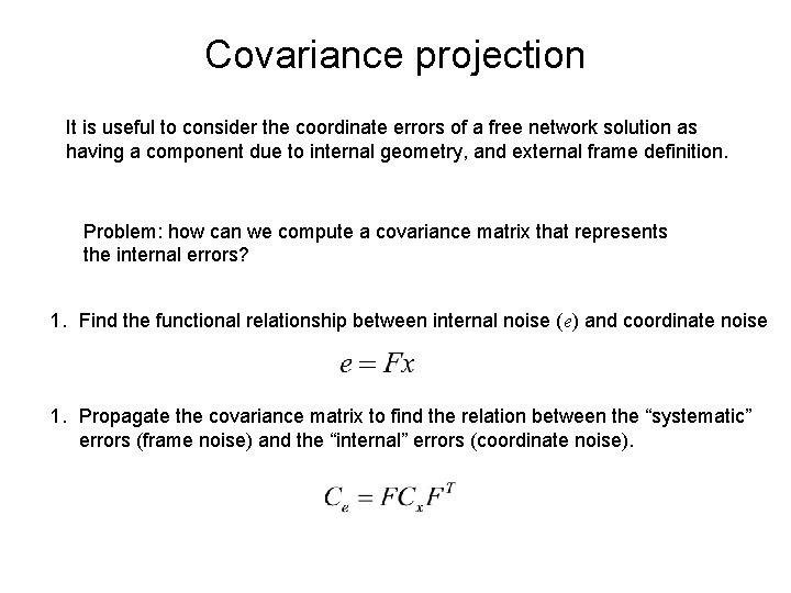
Covariance projection It is useful to consider the coordinate errors of a free network solution as having a component due to internal geometry, and external frame definition. Problem: how can we compute a covariance matrix that represents the internal errors? 1. Find the functional relationship between internal noise (e) and coordinate noise 1. Propagate the covariance matrix to find the relation between the “systematic” errors (frame noise) and the “internal” errors (coordinate noise).

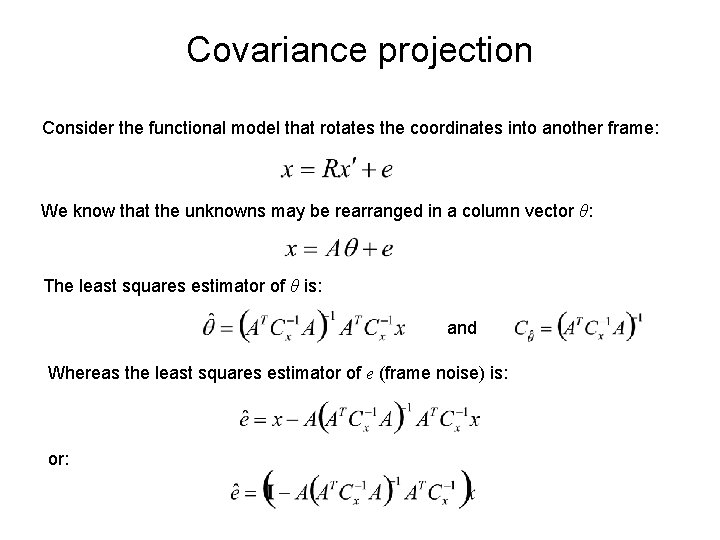
Covariance projection Consider the functional model that rotates the coordinates into another frame: We know that the unknowns may be rearranged in a column vector θ: The least squares estimator of θ is: and Whereas the least squares estimator of e (frame noise) is: or:

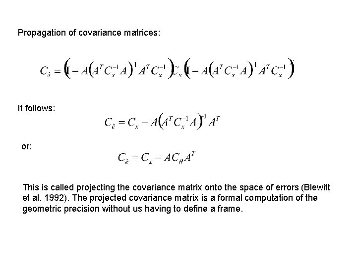
Propagation of covariance matrices: It follows: or: This is called projecting the covariance matrix onto the space of errors (Blewitt et al. 1992). The projected covariance matrix is a formal computation of the geometric precision without us having to define a frame.

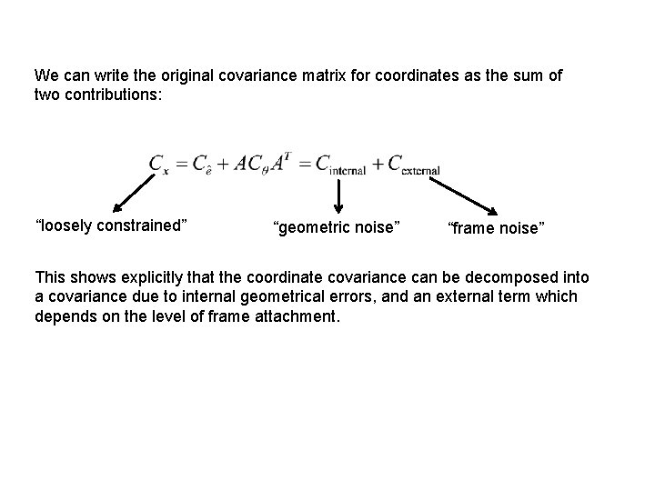
We can write the original covariance matrix for coordinates as the sum of two contributions: “loosely constrained” “geometric noise” “frame noise” This shows explicitly that the coordinate covariance can be decomposed into a covariance due to internal geometrical errors, and an external term which depends on the level of frame attachment.

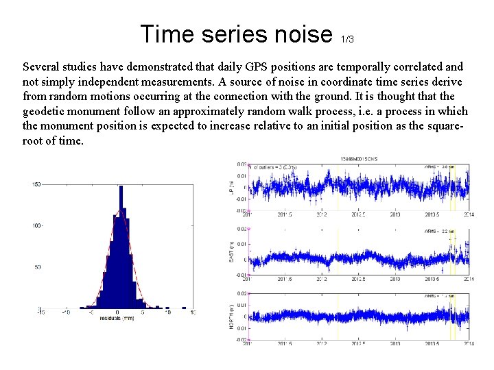
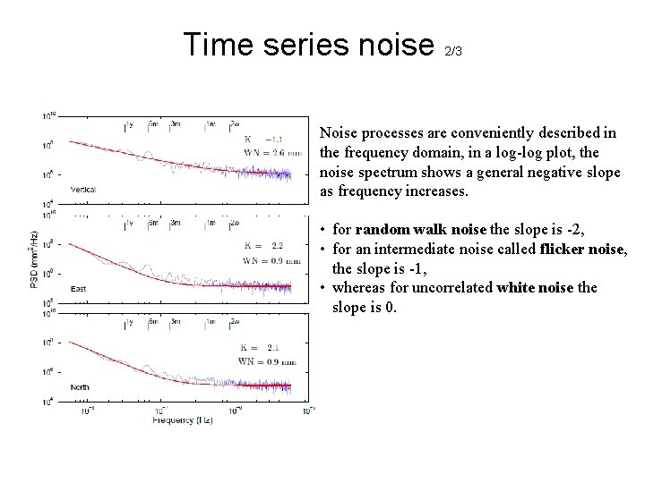
Time series noise 1/3 Several studies have demonstrated that daily GPS positions are temporally correlated and not simply independent measurements. A source of noise in coordinate time series derive from random motions occurring at the connection with the ground. It is thought that the geodetic monument follow an approximately random walk process, i. e. a process in which the monument position is expected to increase relative to an initial position as the squareroot of time.

Time series noise 2/3 Noise processes are conveniently described in the frequency domain, in a log-log plot, the noise spectrum shows a general negative slope as frequency increases. • for random walk noise the slope is -2, • for an intermediate noise called flicker noise, the slope is -1, • whereas for uncorrelated white noise the slope is 0.

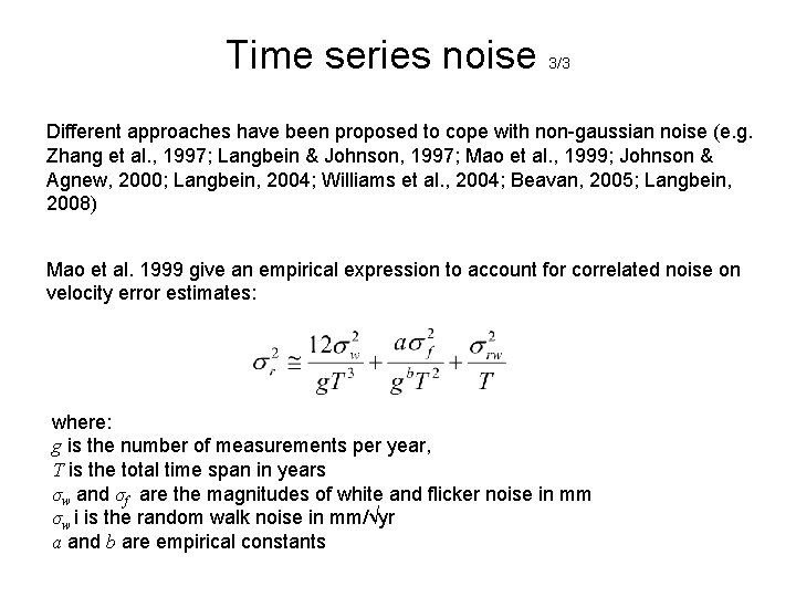
Time series noise 3/3 Different approaches have been proposed to cope with non-gaussian noise (e. g. Zhang et al. , 1997; Langbein & Johnson, 1997; Mao et al. , 1999; Johnson & Agnew, 2000; Langbein, 2004; Williams et al. , 2004; Beavan, 2005; Langbein, 2008) Mao et al. 1999 give an empirical expression to account for correlated noise on velocity error estimates: where: g is the number of measurements per year, T is the total time span in years σw and σf are the magnitudes of white and flicker noise in mm σw i is the random walk noise in mm/√yr a and b are empirical constants

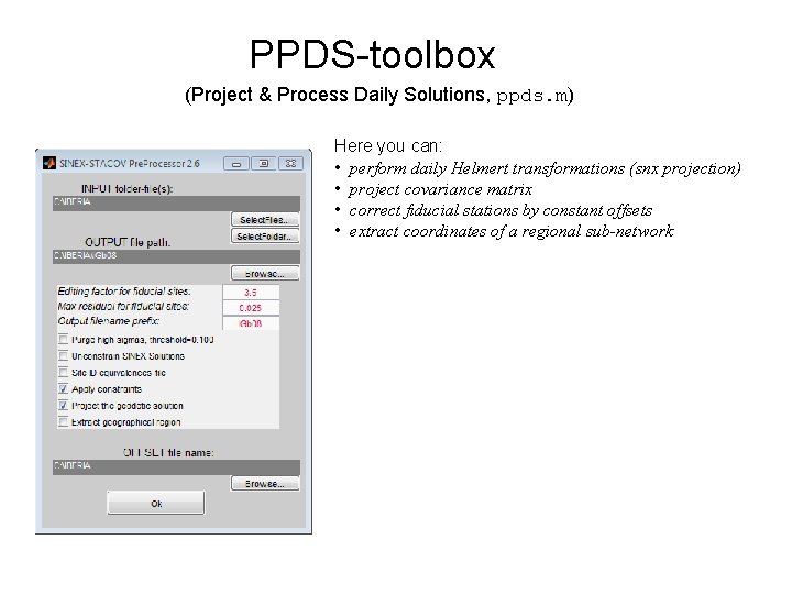
PPDS-toolbox (Project & Process Daily Solutions, ppds. m) Here you can: • perform daily Helmert transformations (snx projection) • project covariance matrix • correct fiducial stations by constant offsets • extract coordinates of a regional sub-network

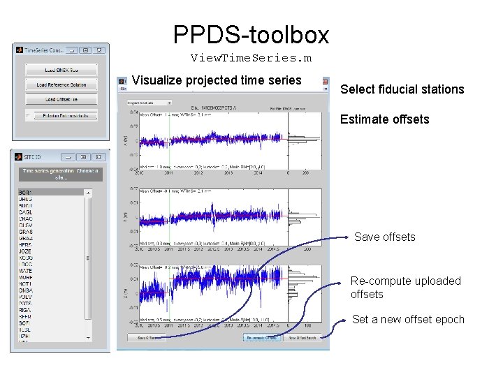
PPDS-toolbox View. Time. Series. m Visualize projected time series Select fiducial stations Estimate offsets Save offsets Re-compute uploaded offsets Set a new offset epoch

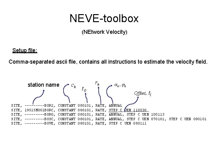
NEVE-toolbox (NEtwork Velocity) Setup file: Comma-separated ascii file, contains all instructions to estimate the velocity field. station name SITE, SITE, -----BOR 2, 19515 M 001 BORC, -----BORG, -----BOSC, -----BOVE, ck CONSTANT CONSTANT t 0 080101, 080101, rk Offset, tl RATE, RATE, ANNUAL STEP C UEN 110530 ANNUAL, STEP C UEN 100113 ANNUAL, STEP C UEN 070101, STEP C UEN 090101 STEP C UEN 080111

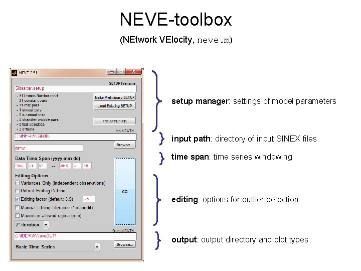
NEVE-toolbox (NEtwork VElocity, neve. m) setup manager: settings of model parameters input path: directory of input SINEX files time span: time series windowing editing: options for outlier detection output: output directory and plot types

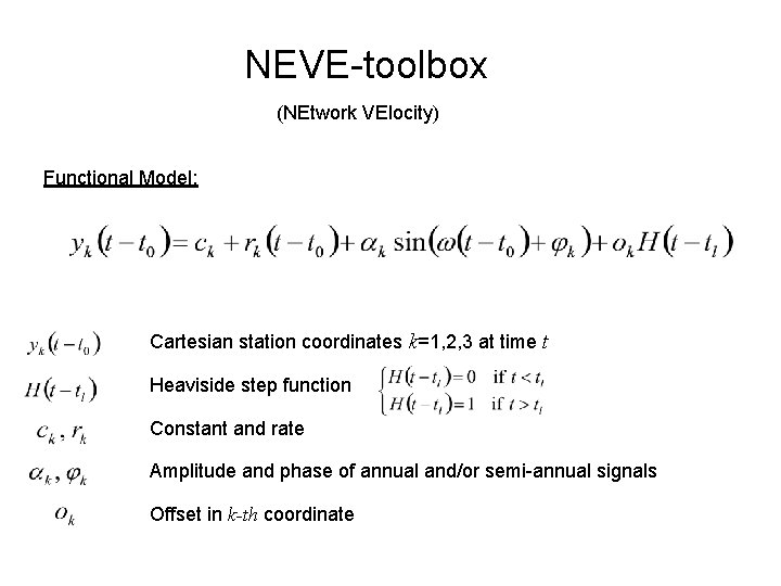
NEVE-toolbox (NEtwork VElocity) Functional Model: Cartesian station coordinates k=1, 2, 3 at time t Heaviside step function Constant and rate Amplitude and phase of annual and/or semi-annual signals Offset in k-th coordinate

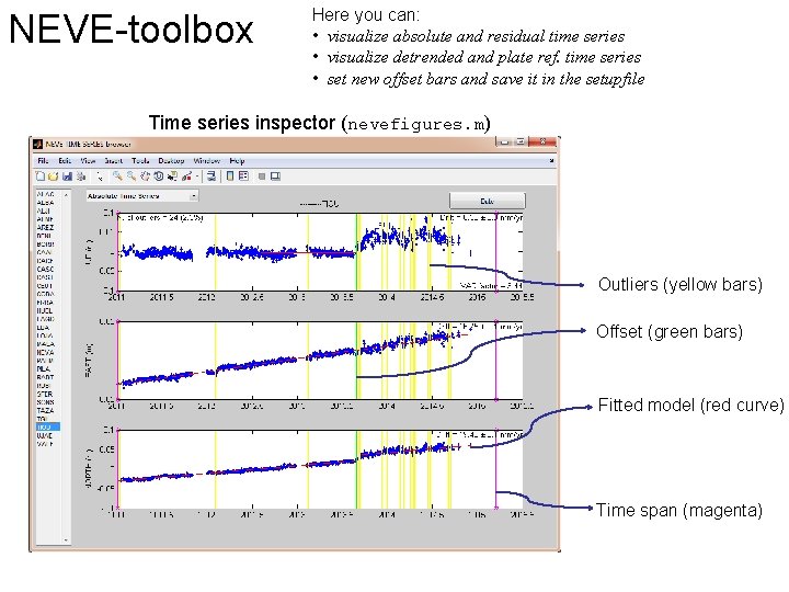
NEVE-toolbox Here you can: • visualize absolute and residual time series • visualize detrended and plate ref. time series • set new offset bars and save it in the setupfile Time series inspector (nevefigures. m) Outliers (yellow bars) Offset (green bars) Fitted model (red curve) Time span (magenta)