Estimation of GLMs Least Squares and Least Other

Estimation of GLMs – Least Squares and Least Other Things Fundamentals of Multivariate Modeling Online Lecture #5 EPSY 905: Least Squares Estimation

Today’s Class • An introduction to estimation…#wtftemplin • Least squares estimation for GLMs • Other “least” type estimators for GLMs Ø “Quantile”/median regression (GLMs) EPSY 905: Least Squares Estimation 2

Why Estimation is Important • In “applied” statistics courses, estimation is not discussed very frequently Ø • Can be very technical…very intimidating Estimation is of critical importance Quality and validity of estimates (and of inferences made from them) depends on how they were obtained Ø New estimation methods appear from time to time and get widespread use without anyone asking whether or not they are any good Ø • Consider an absurd example: I say the mean for IQ should be 20 – just from what I feel Ø Do you believe me? Do you feel like reporting this result? Ø w Estimators need a basis in reality (in statistical theory) EPSY 905: Least Squares Estimation 3

How Estimation Works (More or Less) • Most estimation routines do one of three things: 1. Minimize Something: Typically found with names that have “least” in the title. Forms of least squares include “Generalized”, “Ordinary”, “Weighted”, “Diagonally Weighted”, “WLSMV”, and “Iteratively Reweighted. ” Typically the estimator of last resort… 2. Maximize Something: Typically found with names that have “maximum” in the title. Forms include “Maximum likelihood”, “ML”, “Residual Maximum Likelihood” (REML), “Robust ML”. Typically the gold standard of estimators (and next week we’ll see why). 3. Use Simulation to Sample from Something: more recent advances in simulation use resampling techniques. Names include “Bayesian Markov Chain Monte Carlo”, “Gibbs Sampling”, “Metropolis Hastings”, “Metropolis Algorithm”, and “Monte Carlo”. Also used in combinatorics like bootstrapping. Used for complex models where ML is not available or for methods where prior values are needed. EPSY 905: Least Squares Estimation 4

ESTIMATION OF GLMS USING LEAST SQUARES EPSY 905: Least Squares Estimation 5

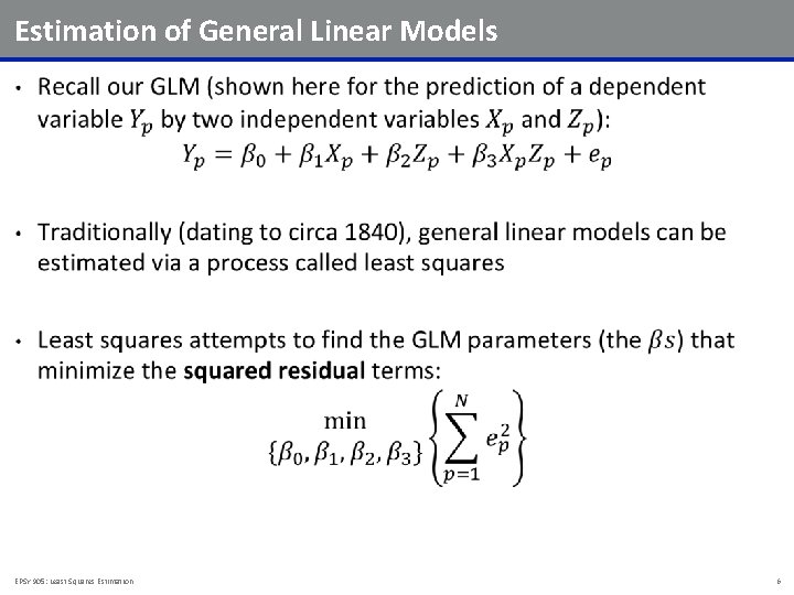
Estimation of General Linear Models • EPSY 905: Least Squares Estimation 6

Where We Are Going (and Why We Are Going There) • EPSY 905: Least Squares Estimation 7

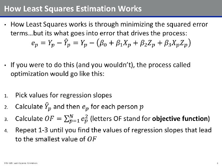
How Least Squares Estimation Works • EPSY 905: Least Squares Estimation 8

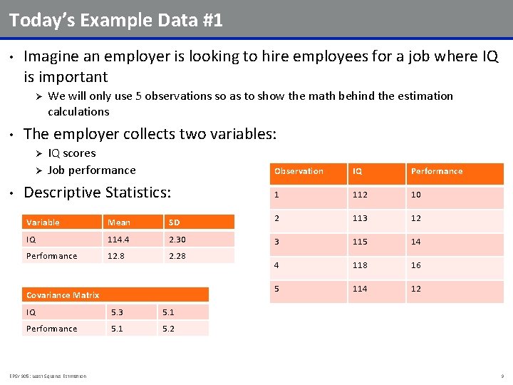
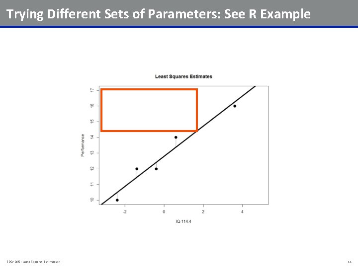
Today’s Example Data #1 • Imagine an employer is looking to hire employees for a job where IQ is important Ø • The employer collects two variables: Ø IQ scores Job performance Observation IQ Performance Descriptive Statistics: 1 112 10 Variable Mean SD 2 113 12 IQ 114. 4 2. 30 3 115 14 Performance 12. 8 2. 28 4 118 16 5 114 12 Ø • We will only use 5 observations so as to show the math behind the estimation calculations Covariance Matrix IQ 5. 3 5. 1 Performance 5. 1 5. 2 EPSY 905: Least Squares Estimation 9

Visualizing the Data EPSY 905: Least Squares Estimation 10

Trying Different Sets of Parameters: See R Example EPSY 905: Least Squares Estimation 11

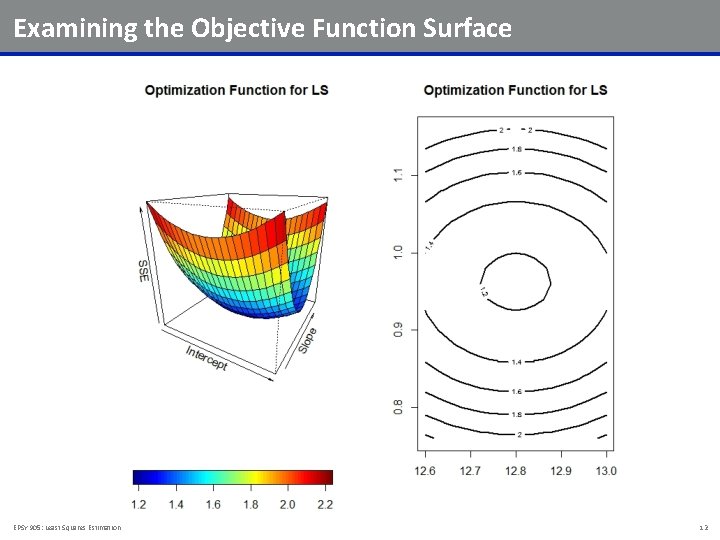
Examining the Objective Function Surface EPSY 905: Least Squares Estimation 12

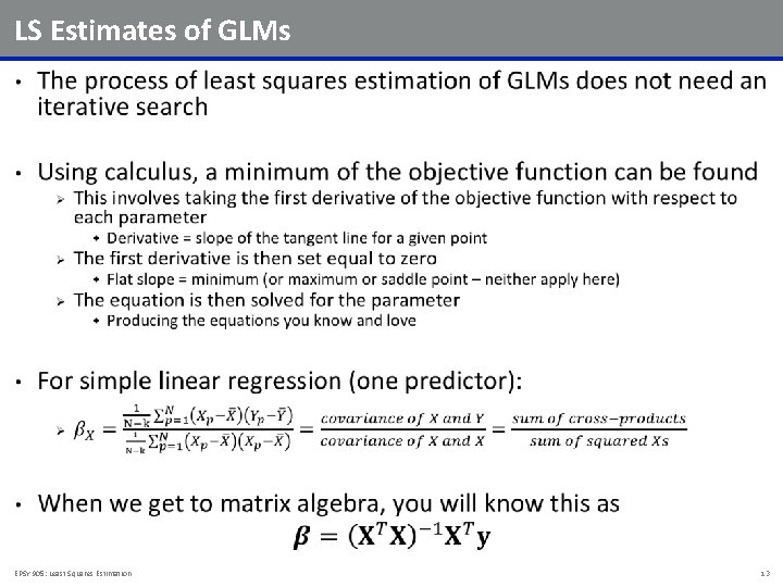
LS Estimates of GLMs • EPSY 905: Least Squares Estimation 13

Ramifications of Closed-Form LS Equations • EPSY 905: Least Squares Estimation 14

Why LS is Still in Use • Least squares estimates still make up the bulk of GLM analyses because: Ø Ø Ø • They are easy to compute They pretty much always give you an answer They have been shown to have good statistical properties The good statistical properties actually come because LS estimates of GLMs match the Maximum Likelihood Estimates Ø Ø We learn more about maximum likelihood estimation in a different lecture For now, know that MLEs are the gold standard when it comes to estimators EPSY 905: Least Squares Estimation 15

Where LS Fails • For all their flexibility, least squares estimates are somewhat limited • When data are not continuous/do not have normally distributed error terms, least squares estimates are not preferred Ø • Some distributions have good estimates (exponential family) but not all For multivariate models with continuous data (repeated measures, longitudinal data, scales of any sort), least squares estimates quickly do not work Ø Ø Cannot handle missing outcomes (deletes entire case) Limited in the types of ways of modeling covariance between observations EPSY 905: Least Squares Estimation 16

OTHER TYPES OF “LEAST” ESTIMATORS: ROBUST GLMS EPSY 905: Least Squares Estimation 17

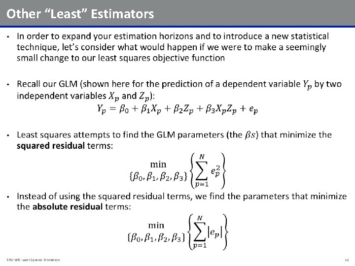
Other “Least” Estimators • EPSY 905: Least Squares Estimation 18

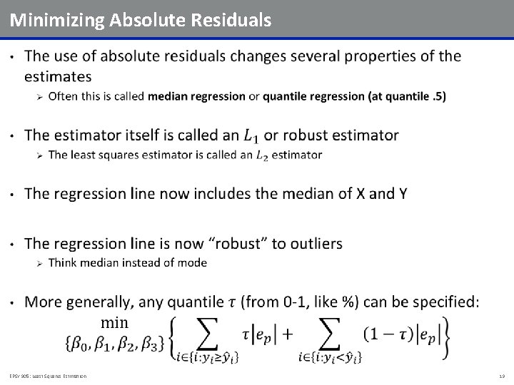
Minimizing Absolute Residuals • EPSY 905: Least Squares Estimation 19

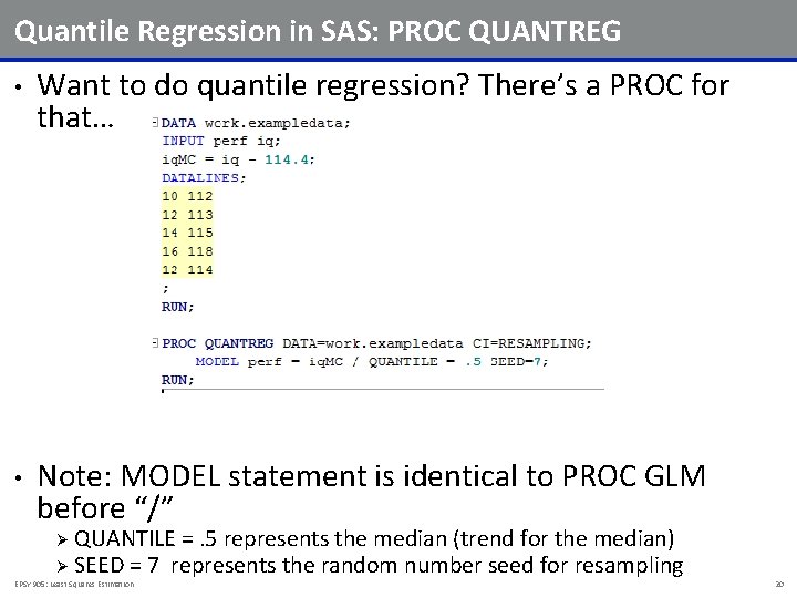
Quantile Regression in SAS: PROC QUANTREG • Want to do quantile regression? There’s a PROC for that… • Note: MODEL statement is identical to PROC GLM before “/” QUANTILE =. 5 represents the median (trend for the median) Ø SEED = 7 represents the random number seed for resampling Ø EPSY 905: Least Squares Estimation 20

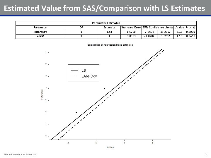
Estimated Value from SAS/Comparison with LS Estimates Parameter Intercept iq. MC EPSY 905: Least Squares Estimation DF 1 1 Parameter Estimates Estimate Standard Error 95% Confidence Limits t Value Pr > |t| 12. 4 1. 5208 7. 5603 17. 2397 8. 15 0. 0039 1 0. 8863 -1. 8207 3. 8207 1. 13 0. 3413 21

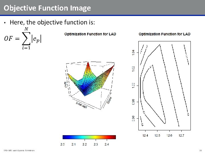
Objective Function Image • EPSY 905: Least Squares Estimation 22

Mathematical Issues with Quantile Regression • EPSY 905: Least Squares Estimation 23

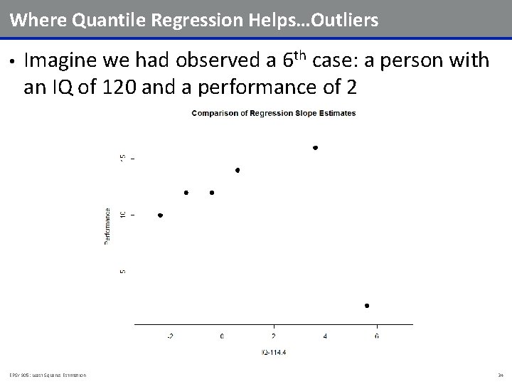
Where Quantile Regression Helps…Outliers • Imagine we had observed a 6 th case: a person with an IQ of 120 and a performance of 2 EPSY 905: Least Squares Estimation 24

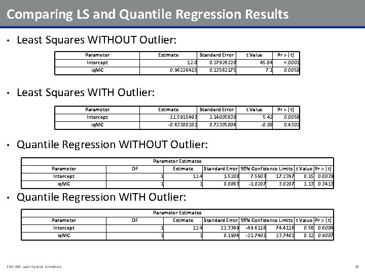
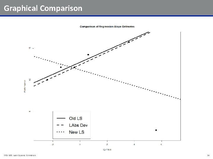
Comparing LS and Quantile Regression Results • Least Squares WITHOUT Outlier: Parameter Intercept iq. MC • Estimate 12. 8 0. 96226415 Estimate Standard Error 11. 5915493 2. 14005638 -0. 63380282 0. 72305804 t Value 5. 42 -0. 88 Pr > |t| 0. 0056 0. 4302 Quantile Regression WITHOUT Outlier: Parameter Intercept iq. MC • t Value Pr > |t| 45. 84 <. 0001 7. 1 0. 0058 Least Squares WITH Outlier: Parameter Intercept iq. MC • Standard Error 0. 27926228 0. 13562175 DF Parameter Estimates Estimate Standard Error 95% Confidence Limits t Value Pr > |t| 1 12. 4 1. 5208 7. 5603 17. 2397 8. 15 0. 0039 1 1 0. 8863 -1. 8207 3. 8207 1. 13 0. 3413 Quantile Regression WITH Outlier: Parameter Intercept iq. MC EPSY 905: Least Squares Estimation DF Parameter Estimates Estimate Standard Error 95% Confidence Limits t Value Pr > |t| 1 12. 4 22. 3349 -49. 6116 74. 4116 0. 56 0. 6084 1 1 8. 1904 -21. 7401 23. 7401 0. 12 0. 9087 25

Graphical Comparison EPSY 905: Least Squares Estimation 26

QUANTILE REGRESSION EXAMPLE EPSY 905: Least Squares Estimation 27

Using Quantile Regression • Quantile regression is a useful research tool for: Ø Ø Ø • Quantile regression cannot help: Ø Ø • When data are skewed Influential (potentially outlying) observations are present Interactions between your IVs and your DV Dependency within or between cases Non-constant variance of residual terms Note: the data for this example are not public. The example is conducted in SAS using PROC QUANTREG Ø The quantreg package in R is similar EPSY 905: Least Squares Estimation 28

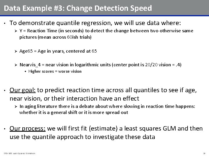
Data Example #3: Change Detection Speed • To demonstrate quantile regression, we will use data where: Ø Y = Reaction Time (in seconds) to detect the change between two otherwise same pictures (mean across 60 ish trials) Ø Age 65 = Age in years, centered at 65 Ø Nearvis_4 = near vision in logarithmic units (center point is 20/20 vision =. 4) w • Our goal: to predict reaction time across all quantiles to see if age, near vision, or their interaction have an effect Ø • Higher scores = worse vision In aging literature there is a debate about where slowing in reaction time happens: whether it is a general shift or it is more spread out Our process: we will first fit (estimate) a least squares GLM and then use the quantile approach to investigate these data EPSY 905: Least Squares Estimation 29

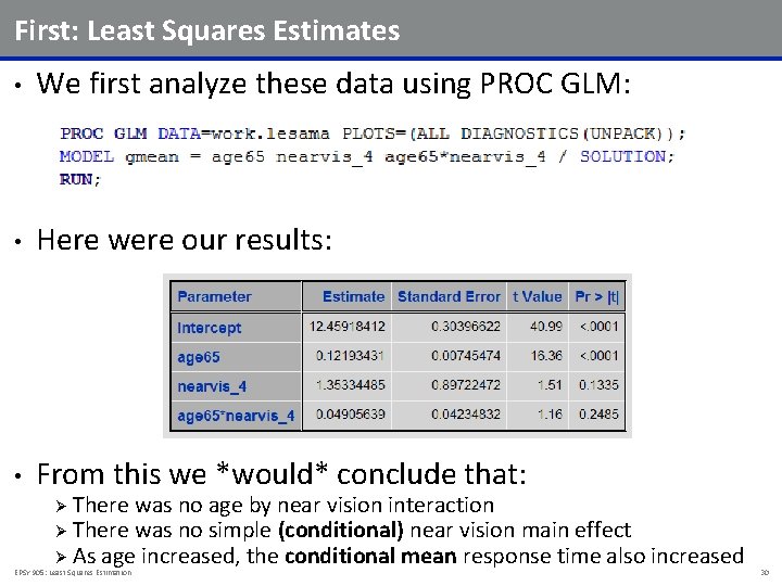
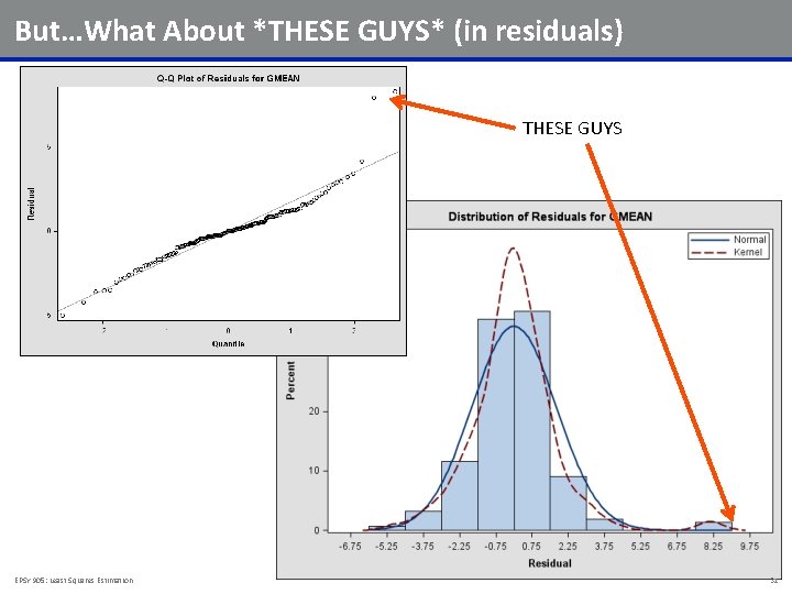
First: Least Squares Estimates • We first analyze these data using PROC GLM: • Here were our results: • From this we *would* conclude that: There was no age by near vision interaction Ø There was no simple (conditional) near vision main effect Ø As age increased, the conditional mean response time also increased Ø EPSY 905: Least Squares Estimation 30

But…What About *THESE GUYS* (in residuals) THESE GUYS EPSY 905: Least Squares Estimation 31

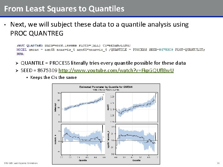
From Least Squares to Quantiles • Next, we will subject these data to a quantile analysis using PROC QUANTREG Ø Ø QUANTILE = PROCESS literally tries every quantile possible for these data SEED = 8675309 http: //www. youtube. com/watch? v=Fkp. GQUfl. Bw. U w Keeps the CIs the same EPSY 905: Least Squares Estimation 32

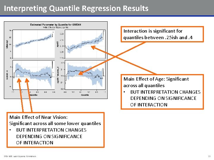
Interpreting Quantile Regression Results Interaction is significant for quantiles between. 25 ish and. 4 Main Effect of Age: Significant across all quantiles • BUT INTERPRETATION CHANGES DEPENDING ON SIGNIFICANCE OF INTERACTION Main Effect of Near Vision: Significant across all some lower quantiles • BUT INTERPRETATION CHANGES DEPENDING ON SIGNIFICANCE OF INTERACTION EPSY 905: Least Squares Estimation 33

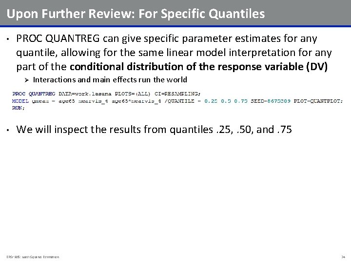
Upon Further Review: For Specific Quantiles • PROC QUANTREG can give specific parameter estimates for any quantile, allowing for the same linear model interpretation for any part of the conditional distribution of the response variable (DV) Ø • Interactions and main effects run the world We will inspect the results from quantiles. 25, . 50, and. 75 EPSY 905: Least Squares Estimation 34

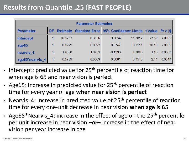
Results from Quantile. 25 (FAST PEOPLE) • • Intercept: predicted value for 25 th percentile of reaction time for when age is 65 and near vision is perfect Age 65: increase in predicted value for 25 th percentile of reaction time for every year of age when near vision is perfect Nearvis_4: increase in predicted value of 25 th percentile of reaction time for every one-unit decrease in near vision when age is 65 Age 65*Nearvis_4: increase in the effect of age on the 25 th percentile per unit increase in near vision –or– increase in the effect of near vision per year increase in age EPSY 905: Least Squares Estimation 35

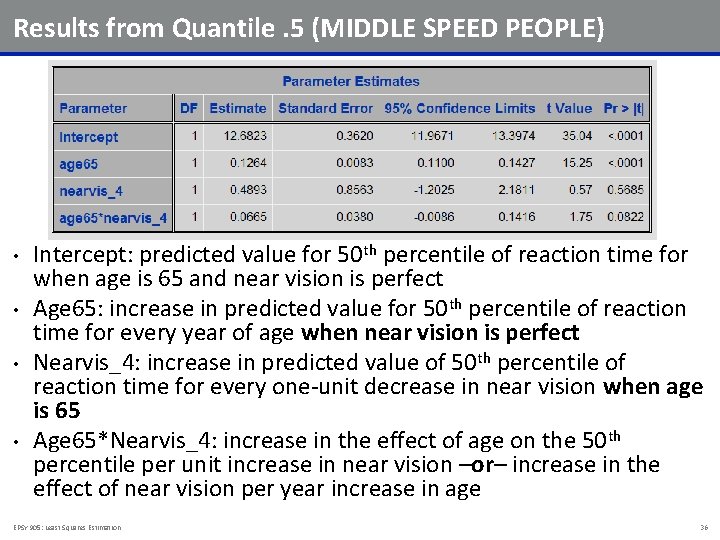
Results from Quantile. 5 (MIDDLE SPEED PEOPLE) • • Intercept: predicted value for 50 th percentile of reaction time for when age is 65 and near vision is perfect Age 65: increase in predicted value for 50 th percentile of reaction time for every year of age when near vision is perfect Nearvis_4: increase in predicted value of 50 th percentile of reaction time for every one-unit decrease in near vision when age is 65 Age 65*Nearvis_4: increase in the effect of age on the 50 th percentile per unit increase in near vision –or– increase in the effect of near vision per year increase in age EPSY 905: Least Squares Estimation 36

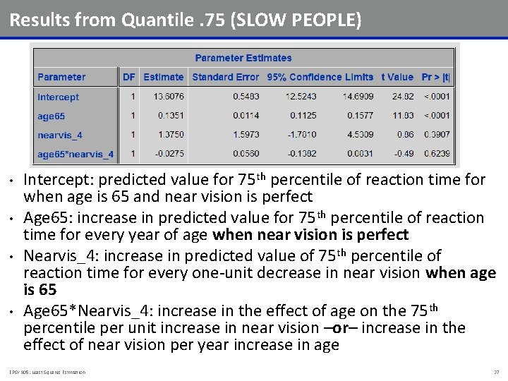
Results from Quantile. 75 (SLOW PEOPLE) • • Intercept: predicted value for 75 th percentile of reaction time for when age is 65 and near vision is perfect Age 65: increase in predicted value for 75 th percentile of reaction time for every year of age when near vision is perfect Nearvis_4: increase in predicted value of 75 th percentile of reaction time for every one-unit decrease in near vision when age is 65 Age 65*Nearvis_4: increase in the effect of age on the 75 th percentile per unit increase in near vision –or– increase in the effect of near vision per year increase in age EPSY 905: Least Squares Estimation 37

QUANTILE REGRESSION IN OTHER FIELDS EPSY 905: Least Squares Estimation 38

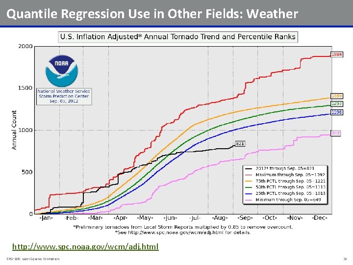
Quantile Regression Use in Other Fields: Weather http: //www. spc. noaa. gov/wcm/adj. html EPSY 905: Least Squares Estimation 39

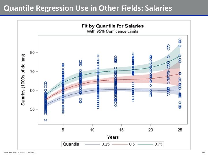
Quantile Regression Use in Other Fields: Salaries EPSY 905: Least Squares Estimation 40

WRAPPING UP EPSY 905: Least Squares Estimation 41

Wrapping Up • This lecture was about estimation, and in the process showed how differing estimators can give you different statistics and results • The key today was to shake your statistical view point: Ø • There are many more ways to arrive at statistical results than you may know Remember: not all estimators are created equal Ø Ø If ever presented with estimates: ask how the numbers were attained If ever getting estimates: get the best you can with your data EPSY 905: Least Squares Estimation 42