PSP Calculations least squares size least squares time

PSP Calculations least squares size, least squares time confidence interval (range), Methods A, B, C, and D CS 1813 Discrete Mathematics, Univ Oklahoma Copyright © 2000 by Rex Page 1

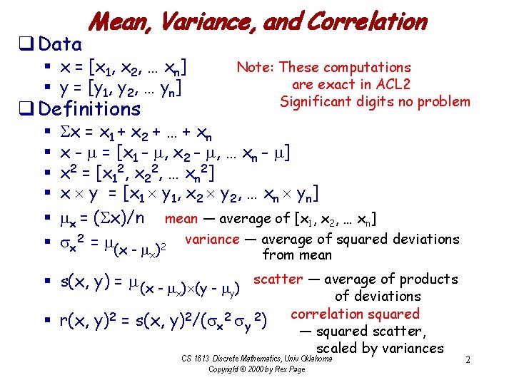
q Data Mean, Variance, and Correlation § x = [x 1, x 2, … xn] § y = [y 1, y 2, … yn] q Definitions § § § Note: These computations are exact in ACL 2 Significant digits no problem x = x 1 + x 2 + … + xn x - = [x 1 - , x 2 - , … xn - ] x 2 = [x 12, x 22, … xn 2] x y = [x 1 y 1, x 2 y 2, … xn yn] x = ( x)/n mean — average of [x 1, x 2, … xn] x 2 = (x - )2 variance — average of squared deviations x from mean § s(x, y) = (x - ) (y - ) scatter — average of products x y of deviations § r(x, y)2 = s(x, y)2/( x 2 y 2) correlation squared — squared scatter, scaled by variances CS 1813 Discrete Mathematics, Univ Oklahoma Copyright © 2000 by Rex Page 2

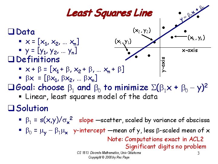
0 + x Least Squares Line 2 § x = [x 1, x 2, … xn] § y = [y 1, y 2, … yn] q Definitions 1 1 2 k 1 § x + = [x 1 + , x 2 + , … xn + ] § x = [ x 1, x 2, … xn] k y-axis q Data • = • y • • • (x , y ) • x-axis • • • q Goal: choose 1 and 0 to minimize ( 1 x + 0 - y)2 § Linear, least squares model of the data q Solution § 1 = s(x, y)/ x 2 slope —scatter, scaled by variance of abscissa § 0 = y - 1 x y-intercept —mean of y, less -scaled mean of x Note: Computations exact in ACL 2 Significant digits no problem CS 1813 Discrete Mathematics, Univ Oklahoma Copyright © 2000 by Rex Page 3

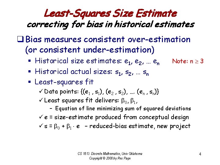
Least-Squares Size Estimate correcting for bias in historical estimates q Bias measures consistent over-estimation (or consistent under-estimation) § Historical size estimates: e 1, e 2, … en § Historical actual sizes: s 1, s 2, … sn § Least-squares fit Note: n 3 ü Data points: {(e 1 , s 1), (e 2 , s 2), …. (en , sn)} ü Least squares fit delivers: 0, 1, – Equation of line minimizing sum of squared deviations ü e = size-estimate produced from conceptual design ü s = 0 + 1 e – reduced-bias estimate, new project CS 1813 Discrete Mathematics, Univ Oklahoma Copyright © 2000 by Rex Page 4

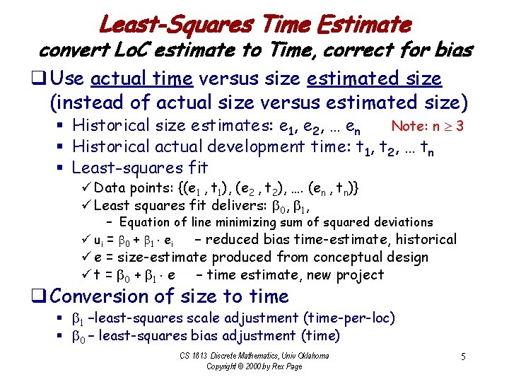
Least-Squares Time Estimate convert Lo. C estimate to Time, correct for bias q Use actual time versus size estimated size (instead of actual size versus estimated size) § Historical size estimates: e 1, e 2, … en Note: n 3 § Historical actual development time: t 1, t 2, … tn § Least-squares fit ü Data points: {(e 1 , t 1), (e 2 , t 2), …. (en , tn)} ü Least squares fit delivers: 0, 1, – Equation of line minimizing sum of squared deviations ü ui = 0 + 1 e i – reduced bias time-estimate, historical ü e = size-estimate produced from conceptual design ü t = 0 + 1 e – time estimate, new project q Conversion of size to time § 1 –least-squares scale adjustment (time-per-loc) § 0 – least-squares bias adjustment (time) CS 1813 Discrete Mathematics, Univ Oklahoma Copyright © 2000 by Rex Page 5

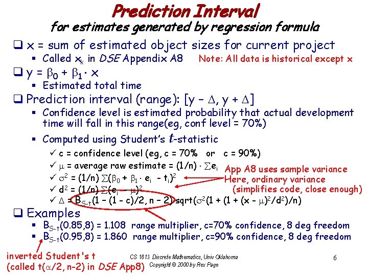
Prediction Interval for estimates generated by regression formula q x = sum of estimated object sizes for current project § Called xk in DSE Appendix A 8 q y = 0 + 1 x Note: All data is historical except x § Estimated total time q Prediction interval (range): [y – D, y + D] § Confidence level is estimated probability that actual development time will fall in this range(eg, conf level = 70%) § Computed using Student’s t-statistic ü c = confidence level (eg, c = 70% or c = 90%) ü = average raw estimate = (1/n) ei App A 8 uses sample variance ü 2 = (1/n) ( 0 + 1 ei - ti)2 Here, ordinary variance 2 2 (simplifies code, close enough) ü d = (1/n) (ei - ) ü D = BS-t(1 – (1 - c)/2, n – 2) sqrt( 2(1 + (x - )2/d 2)/n) q Examples § BS-t(0. 85, 8) = 1. 108 range multiplier, c=70% confidence, 8 deg freedom § BS-t(0. 95, 8) = 1. 860 range multiplier, c=90% confidence, 8 deg freedom inverted Student's t CS 1813 Discrete Mathematics, Univ Oklahoma (called t(a/2, n-2) in DSE App 8) Copyright © 2000 by Rex Page 6

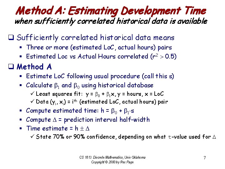
Method A: Estimating Development Time when sufficiently correlated historical data is available q Sufficiently correlated historical data means § Three or more (estimated Lo. C, actual hours) pairs § Estimated Loc vs Actual Hours correlated (r 2 > 0. 5) q Method A § Estimate Lo. C following usual procedure (call this s) § Calculate 1 and 0 using historical database ü Least squares fit: y = 0 + 1 x, y = hours, x = Lo. C ü Data (yi, xi) = ith (estimated Lo. C, actual hours) pair § Compute estimated time: h = 0 + 1 s § Compute D = prediction interval half-width § Time estimate = h D ü State 70% or 90% confidence, depending on what t-value used for D CS 1813 Discrete Mathematics, Univ Oklahoma Copyright © 2000 by Rex Page 7

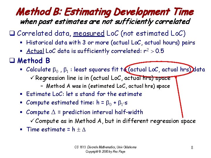
Method B: Estimating Development Time when past estimates are not sufficiently correlated q Correlated data, measured Lo. C (not estimated Lo. C) § Historical data with 3 or more (actual Lo. C, actual hours) pairs § Actual Lo. C data is sufficiently correlated: r 2 > 0. 5 q Method B § Calculate 0 , 1 : least squares fit to (actual Lo. C, actual hrs) data ü Regression line is in (actual Lo. C, actual hrs) space – Method A was in (estimated Lo. C, actual hrs) space § Estimate Lo. C: let s stand for the estimate § Compute estimated time: h = 0 + 1 s § Compute D = prediction interval half-width ü Compute as in Method A, but in different regression space § Time estimate = h D CS 1813 Discrete Mathematics, Univ Oklahoma Copyright © 2000 by Rex Page 8

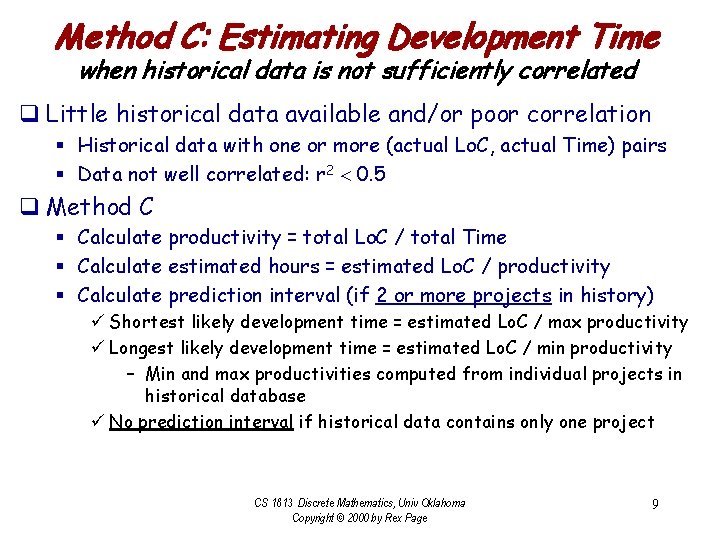
Method C: Estimating Development Time when historical data is not sufficiently correlated q Little historical data available and/or poor correlation § Historical data with one or more (actual Lo. C, actual Time) pairs § Data not well correlated: r 2 < 0. 5 q Method C § Calculate productivity = total Lo. C / total Time § Calculate estimated hours = estimated Lo. C / productivity § Calculate prediction interval (if 2 or more projects in history) ü Shortest likely development time = estimated Lo. C / max productivity ü Longest likely development time = estimated Lo. C / min productivity – Min and max productivities computed from individual projects in historical database ü No prediction interval if historical data contains only one project CS 1813 Discrete Mathematics, Univ Oklahoma Copyright © 2000 by Rex Page 9

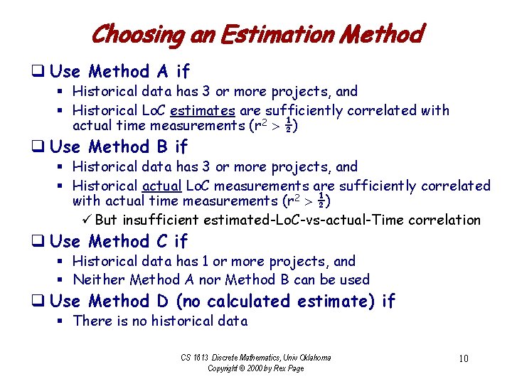
Choosing an Estimation Method q Use Method A if § Historical data has 3 or more projects, and § Historical Lo. C estimates are sufficiently correlated with actual time measurements (r 2 > ½) q Use Method B if § Historical data has 3 or more projects, and § Historical actual Lo. C measurements are sufficiently correlated with actual time measurements (r 2 > ½) ü But insufficient estimated-Lo. C-vs-actual-Time correlation q Use Method C if § Historical data has 1 or more projects, and § Neither Method A nor Method B can be used q Use Method D (no calculated estimate) if § There is no historical data CS 1813 Discrete Mathematics, Univ Oklahoma Copyright © 2000 by Rex Page 10

The End CS 1813 Discrete Mathematics, Univ Oklahoma Copyright © 2000 by Rex Page 11