Gaussian Elimination Simultaneous equations splines least squares fitting

Gaussian Elimination Simultaneous equations, splines, least squares fitting

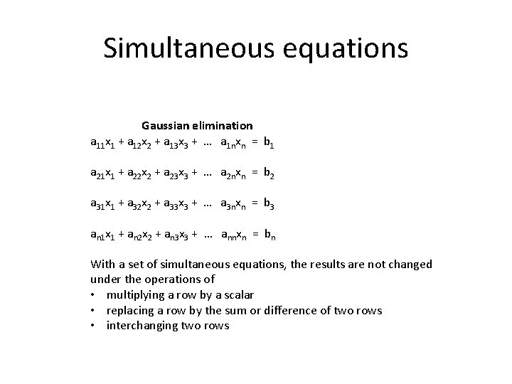
Simultaneous equations Gaussian elimination a 11 x 1 + a 12 x 2 + a 13 x 3 + … a 1 nxn = b 1 a 21 x 1 + a 22 x 2 + a 23 x 3 + … a 2 nxn = b 2 a 31 x 1 + a 32 x 2 + a 33 x 3 + … a 3 nxn = b 3 an 1 x 1 + an 2 x 2 + an 3 x 3 + … annxn = bn With a set of simultaneous equations, the results are not changed under the operations of • multiplying a row by a scalar • replacing a row by the sum or difference of two rows • interchanging two rows

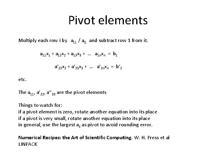
Pivot elements Multiply each row i by a 11 / ai 1 and subtract row 1 from it. a 11 x 1 + a 12 x 2 + a 13 x 3 + … a 1 nxn = b 1 a’ 22 x 2 + a’ 23 x 3 + … a’ 2 nxn = b’ 2 etc. The a 11, a’ 22, a’’ 33 are the pivot elements Things to watch for: if a pivot element is zero, rotate another equation into its place if a pivot is very small, rotate another equation into its place in general, use the largest aii as pivot to avoid rounding error. Numerical Recipes: the Art of Scientific Computing. W. H. Press et al LINPACK

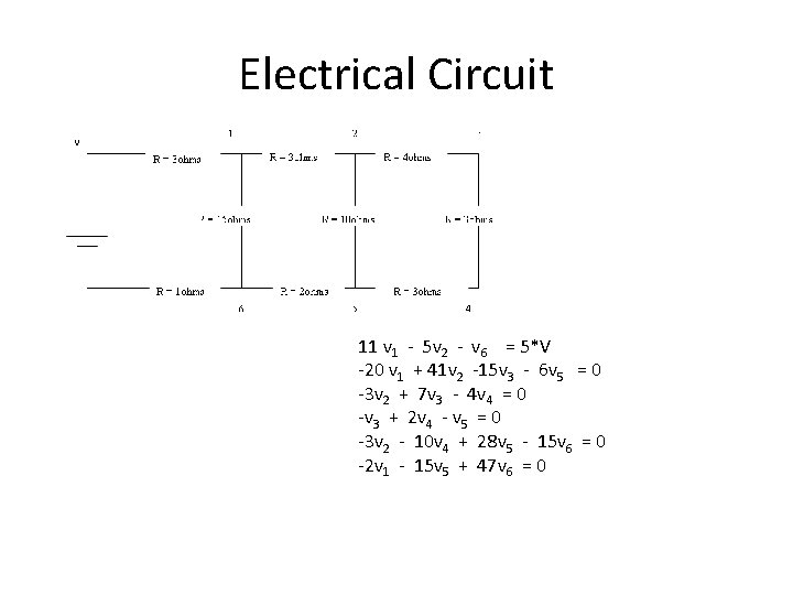
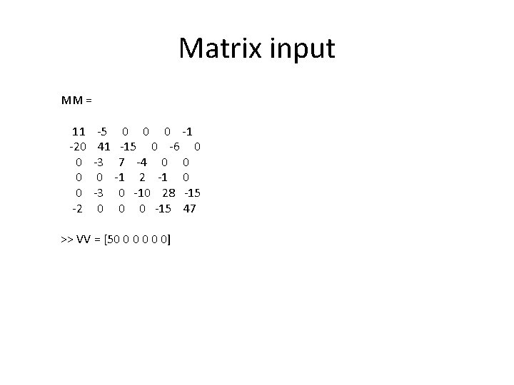
Electrical Circuit 11 v 1 - 5 v 2 - v 6 = 5*V -20 v 1 + 41 v 2 -15 v 3 - 6 v 5 = 0 -3 v 2 + 7 v 3 - 4 v 4 = 0 -v 3 + 2 v 4 - v 5 = 0 -3 v 2 - 10 v 4 + 28 v 5 - 15 v 6 = 0 -2 v 1 - 15 v 5 + 47 v 6 = 0

Matrix input MM = 11 -5 0 0 0 -1 -20 41 -15 0 -6 0 0 -3 7 -4 0 0 -1 2 -1 0 0 -3 0 -10 28 -15 -2 0 0 0 -15 47 >> VV = [50 0 0 0]

splines

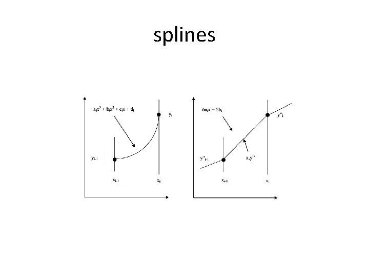
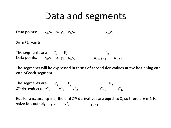
Data and segments Data points: x 0, y 0 x 1, y 1 x 2, y 2 xn, yn So, n+1 points The segments are P 1 P 2 Pn Data points: x 0, y 0 x 1, y 1 x 2, y 2 xn-1, yn-1 xn, yn The segments will be expressed in terms of second derivatives at the beginning and end of each segment: The segments are P 1 P 2 Pn 2 nd derivatives: y” 0 y” 1 y” 2 y”n-1 y”n But for a natural spline, the end 2 nd derivatives are equal to 0, so there are n-1 to solve for, namely y” 1 y” 2 y”n-1

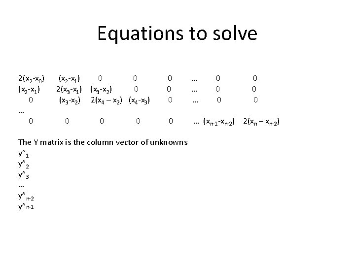
Equations to solve 2(x 2 -x 0) (x 2 -x 1) 0 … 0 (x 2 -x 1) 2(x 3 -x 1) (x 3 -x 2) 0 … 0 0 (x 3 -x 2) 2(x 4 – x 2) (x 4 -x 3) 0 … 0 … 0 0 … (xn-1 -xn-2) 2(xn – xn-2) The Y matrix is the column vector of unknowns y” 1 y” 2 y” 3 … y”n-2 y”n-1

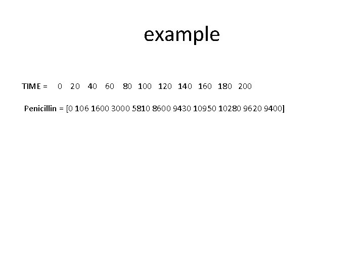
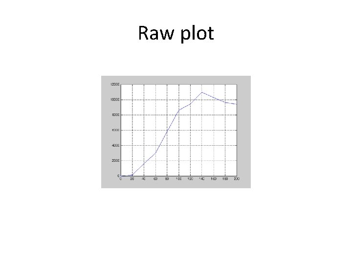
example TIME = 0 20 40 60 80 100 120 140 160 180 200 Penicillin = [0 106 1600 3000 5810 8600 9430 10950 10280 9620 9400]

Raw plot

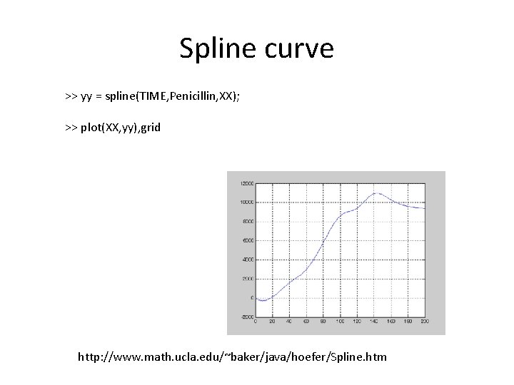
Spline curve >> yy = spline(TIME, Penicillin, XX); >> plot(XX, yy), grid http: //www. math. ucla. edu/~baker/java/hoefer/Spline. htm

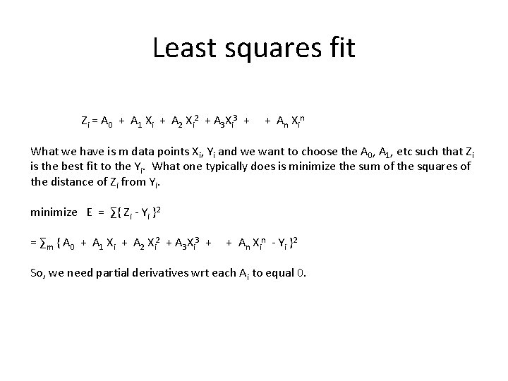
Least squares fit Zi = A 0 + A 1 Xi + A 2 Xi 2 + A 3 Xi 3 + + An Xin What we have is m data points Xi, Yi and we want to choose the A 0, A 1, etc such that Zi is the best fit to the Yi. What one typically does is minimize the sum of the squares of the distance of Zi from Yi. minimize E = ∑{ Zi - Yi }2 = ∑m { A 0 + A 1 Xi + A 2 Xi 2 + A 3 Xi 3 + + An Xin - Yi }2 So, we need partial derivatives wrt each Ai to equal 0.

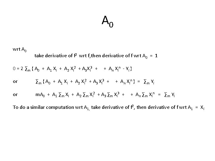
A 0 wrt A 0 take derivative of f 2 wrt f, then derivative of f wrt A 0 = 1 0 = 2 ∑m { A 0 + A 1 Xi + A 2 Xi 2 + A 3 Xi 3 + + An Xin - Yi } or ∑m { A 0 + A 1 Xi + A 2 Xi 2 + A 3 Xi 3 + + An Xin } = ∑m Yi or m. A 0 + A 1 ∑m Xi + A 2 ∑m Xi 2 + A 3 ∑m Xi 3 + + An ∑m Xin = ∑m Yi To do a similar computation wrt A 1, take derivative of f 2, then derivative of f wrt A 1 = Xi

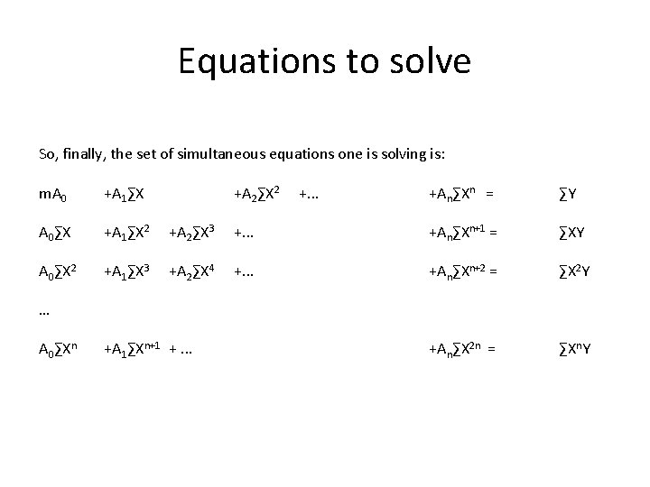
Equations to solve So, finally, the set of simultaneous equations one is solving is: m. A 0 +A 1∑X +A 2∑X 2 +. . . +An∑Xn = A 0∑X +A 1∑X 2 +A 2∑X 3 +. . . +An∑Xn+1 = ∑Y ∑XY A 0∑X 2 … +A 1∑X 3 +A 2∑X 4 +. . . +An∑Xn+2 = ∑X 2 Y A 0∑Xn +A 1∑Xn+1 +. . . +An∑X 2 n = ∑Xn. Y

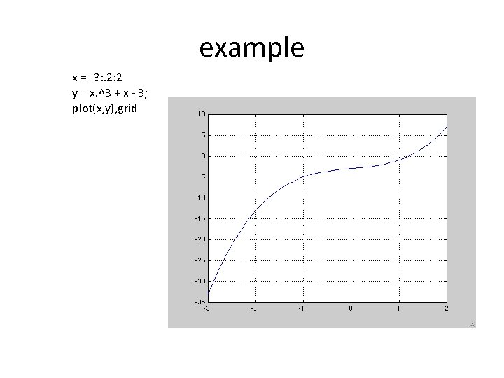
example x = -3: . 2: 2 y = x. ^3 + x - 3; plot(x, y), grid

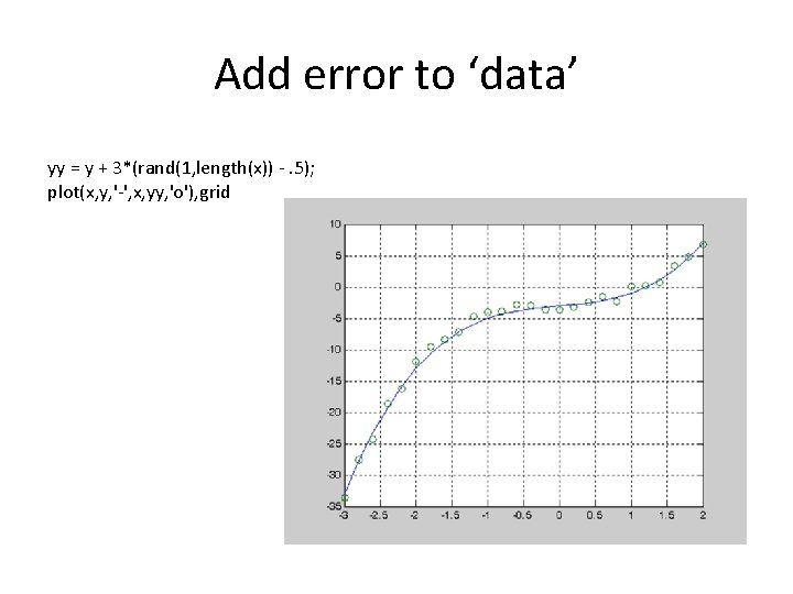
Add error to ‘data’ yy = y + 3*(rand(1, length(x)) -. 5); plot(x, y, '-', x, yy, 'o'), grid

Best fit [p s] = polyfit(x, yy, 3) p = 0. 9737 -0. 0009 1. 1948 -2. 5593 yyy = polyval(p, x); % x could be a different vector than the data values plot(x, y, '-', x, yy, 'o', x, yyy, 'r'), grid

a polyfit version function [ a ] = my. Poly(x, y, n) %n contains polynomial order x = (x(: ). ')'; y = (y(: ). ')'; k = length(x); xp = 0: 1: 2*n; xmat = zeros(k, 2*n); xmat = [ ones(k, 1) xmat]; ymat = repmat(y, 1, n+1); for col = 1: 2*n xmat(: , col+1) = xmat(: , col). *x; end for col = 2: n+1 ymat(: , col) = ymat(: , col-1). *x; end xvec = sum(xmat); yvec = sum(ymat); MM = zeros(n+1, n+1); C = yvec'; for row = 1: n+1 MM(row, : ) = xvec(row: row+n); end a = MMC; end